Syllabus:
Overview of Biological Neurons: Structure of biological neuron, neurobiological analogy, Biological neuron equivalencies to artificial neuron model, Evolution of neural network.
Activation Functions: Threshold functions, Signum function, Sigmoid function, Tan hyperbolic function, Stochastic function, Ramp function, Linear function, Identity function.
ANN Architecture: Feed forward network, Feed backward network, single and multilayer network, fully recurrent network.
PYQ Analysis
High Priority Topics (15 marks questions)
- Biological Neuron Structure - (2024: 15 marks, 2023: 15 marks, 2022: 15 marks)
- Activation Functions - (2024: 15 marks, 2022: 15 marks)
- Applications of Neural Networks - (2023: 15 marks)
Medium Priority Topics (Short answers)
- Role of Dendrites and Axons - 2024 (2.5 marks)
- Applications of Neural Network - 2024 (2.5 marks)
- Activation Function Definition - 2023 (2.5 marks)
- Feedforward vs Feedback Networks - 2023 (2.5 marks)
Low Priority Topics
- Evolution of Neural Network - 2022 (Short answer)
Section 1: Overview of Biological Neurons
1.1 Introduction to Neural Networks
PYQ: Describe the structure of a biological neuron in detail and explain how its components contribute to signal processing and transmission. (2024, 15 marks)
PYQ: How biological neural is different from the artificial neural networks? Explain architecture of biological neural network. (2023, 15 marks)
PYQ: Explain the component of a Biological Neuron. Also focus on Biological neuron equivalencies to artificial neuron model. (2022, 15 marks)
What is a Neural Network?
A Neural Network is a computing system inspired by the human brain. Just like our brain has billions of neurons (nerve cells) that work together to help us think, learn, and make decisions, artificial neural networks have artificial neurons that work together to solve problems.
Why Study Biological Neurons?
To understand artificial neural networks, we first need to understand how real neurons in our brain work. Scientists created artificial neural networks by copying the way biological neurons function.
Real-Life Analogy:
Think of neurons like a network of people passing messages. When you touch something hot:
- Sensors in your hand (neurons) detect heat
- They send signals through a chain of neurons
- The message reaches your brain
- Your brain processes it and sends a signal back
- Your hand moves away from the hot object
All this happens in milliseconds! Artificial neural networks try to copy this amazing ability.
1.2 Structure of Biological Neuron
PYQ: Role of Dendrites and Axons in a Biological Neuron (2024, 2.5 marks)
A biological neuron is a specialized cell in the nervous system that processes and transmits information through electrical and chemical signals. The human brain contains approximately 86 billion neurons, each connected to thousands of other neurons.
Main Components of a Biological Neuron:
ASCII Diagram:
        Dendrites (Input)
            ↓ ↓ ↓
    ┌───────────────────┐
    │                   │
    │    Cell Body      │ ← Nucleus (Processing Center)
    │    (Soma)         │
    │                   │
    └─────────┬─────────┘
              │
              ↓
         Axon (Output)
              │
              ↓
    ┌─────────────────┐
    │  Axon Terminal  │
    │   (Synapses)    │
    └─────────────────┘
              ↓
        Next Neuron
Visual Diagram:

Detailed Components:
1. Dendrites (Input Receivers)
Function: Receive signals from other neurons
How it works:
- Dendrites are like tree branches extending from the cell body
- They receive chemical signals from other neurons
- Multiple dendrites can receive many signals at the same time
- Each dendrite can receive different strength signals
Analogy: Think of dendrites like antennas on your phone that receive signals from different cell towers.
Role in Signal Processing:
- Collect incoming signals from thousands of other neurons
- Convert chemical signals into electrical impulses
- Pass these signals to the cell body for processing
2. Cell Body / Soma (Processing Unit)
Function: Processes all incoming signals
Components:
- Nucleus: Contains genetic information (DNA)
- Cytoplasm: Fluid that fills the cell
- Organelles: Small structures that keep the cell alive
How it works:
- Receives all signals from dendrites
- Adds up all the incoming signals (summation)
- Decides whether to send a signal forward or not
- This decision is based on whether the total signal crosses a threshold
Analogy: Like a calculator that adds up all the numbers and decides if the total is enough to trigger an action.
Role in Signal Processing:
- Integrates all incoming signals
- Performs weighted summation
- Determines if the neuron should "fire" (activate)
3. Axon (Output Transmitter)
Function: Carries the output signal to other neurons
Characteristics:
- Long, thin fiber extending from the cell body
- Can be very short (1mm) or very long (1 meter in some cases)
- Covered with myelin sheath (insulation) for faster transmission
- Carries electrical impulses called "action potentials"
How it works:
- If the cell body decides to activate, an electrical signal travels down the axon
- The signal travels at speeds up to 120 meters per second
- The myelin sheath helps the signal jump quickly along the axon
Analogy: Like an electrical wire that carries current from one point to another.
Role in Signal Transmission:
- Conducts electrical impulses away from the cell body
- Maintains signal strength over long distances
- Ensures rapid communication between neurons
4. Axon Terminals / Synapses (Output Connectors)
Function: Connect to other neurons and transmit signals
How it works:
- At the end of the axon, there are many small branches
- Each branch ends in a synapse (connection point)
- When the electrical signal reaches the synapse, it releases chemicals called neurotransmitters
- These chemicals cross a tiny gap (synaptic cleft) to reach the next neuron's dendrites
Analogy: Like a Bluetooth connection that wirelessly sends data from one device to another.
Role in Signal Transmission:
- Converts electrical signals back to chemical signals
- Releases neurotransmitters into the synaptic gap
- Influences the next neuron's activity
1.3 How Biological Neurons Work (Signal Processing)
Step-by-Step Process:
Step 1: Signal Reception
- Dendrites receive chemical signals (neurotransmitters) from other neurons
- Each signal has a certain strength (weight)
- Some signals are excitatory (encourage firing) - positive
- Some signals are inhibitory (discourage firing) - negative
Step 2: Signal Integration
- The cell body adds up all incoming signals
- This is called "spatial summation" (adding signals from different dendrites)
- Also does "temporal summation" (adding signals arriving at different times)
Step 3: Decision Making
- The cell body has a threshold value
- If total signal > threshold → Neuron fires (sends signal)
- If total signal < threshold → Neuron doesn't fire (no signal)
Step 4: Signal Transmission
- If neuron fires, an electrical impulse (action potential) travels down the axon
- This is an "all-or-nothing" response (either fires completely or doesn't fire at all)
- The signal strength doesn't decrease as it travels
Step 5: Signal Output
- The electrical signal reaches the axon terminals
- Neurotransmitters are released into the synaptic gap
- These chemicals reach the dendrites of the next neurons
- The process repeats
Mathematical Representation:
Total Input = (Signal₁ × Weight₁) + (Signal₂ × Weight₂) + ... + (Signalₙ × Weightₙ)

If Total Input ≥ Threshold:
    Neuron Fires (Output = 1)
Else:
    Neuron Doesn't Fire (Output = 0)
1.4 Biological vs Artificial Neuron
PYQ: How biological neural is different from the artificial neural networks? (2023, 15 marks)
PYQ: Biological neuron equivalencies to artificial neuron model. (2022, 15 marks)
The artificial neuron model is a simplified model of the biological neuron. It is a mathematical model that is used to simulate the behavior of the biological neuron.
Artificial Neuron Model:
Inputs (x₁, x₂, x₃, ..., xₙ)
    ↓
Weights (w₁, w₂, w₃, ..., wₙ)
    ↓
Weighted Sum: Σ(xᵢ × wᵢ) + bias
    ↓
Activation Function
    ↓
Output (y)
Equivalencies Table:
| Biological Component | Artificial Equivalent | Function |
|---|---|---|
| Dendrites | Input connections | Receive signals from other neurons |
| Synaptic Weights | Connection weights (w) | Determine signal strength/importance |
| Cell Body (Soma) | Summation function (Σ) | Adds up all weighted inputs |
| Threshold | Bias/Threshold value | Decision boundary for activation |
| Axon | Output connection | Transmits the result |
| Activation | Activation function | Determines output based on input |
| Synapses | Weights between layers | Connect neurons in different layers |
| Learning | Weight adjustment | Changes connection strengths |
Detailed Comparison:
1. Input Mechanism
Biological:
- Dendrites receive chemical signals (neurotransmitters)
- Multiple dendrites can receive different signals simultaneously
- Signals can be excitatory (+) or inhibitory (-)
Artificial:
- Input nodes receive numerical values
- Each input has an associated weight
- Inputs are multiplied by weights: x₁w₁, x₂w₂, etc.
2. Processing
Biological:
- Cell body integrates all incoming signals
- Performs spatial and temporal summation
- Compares total with threshold
Artificial:
- Summation function: Σ(xᵢwᵢ) + bias
- Bias acts as threshold adjustment
- Result passed to activation function
3. Activation
Biological:
- All-or-nothing response (action potential)
- Either fires completely or doesn't fire
- Fixed amplitude, variable frequency
Artificial:
- Activation function determines output
- Can be binary (0/1) or continuous (0 to 1)
- Various functions: sigmoid, tanh, ReLU, etc.
4. Output
Biological:
- Electrical impulse travels down axon
- Neurotransmitters released at synapses
- Signal transmitted to multiple neurons
Artificial:
- Single numerical output value
- Passed to next layer of neurons
- Can connect to multiple neurons
5. Learning
Biological:
- Synaptic plasticity (connections strengthen or weaken)
- "Neurons that fire together, wire together"
- Long-term potentiation and depression
Artificial:
- Weight adjustment through training
- Backpropagation algorithm
- Gradient descent optimization
Key Differences:
| Aspect | Biological | Artificial |
|---|---|---|
| Speed | Milliseconds (slow) | Nanoseconds (fast) |
| Connections | ~10,000 per neuron | Typically fewer |
| Energy | Very efficient | Requires more power |
| Fault Tolerance | High (brain adapts) | Low (needs retraining) |
| Parallelism | Massive parallel processing | Limited parallelism |
| Learning | Continuous, lifelong | Discrete training phases |
| Size | Microscopic | Virtual/software |
1.5 Evolution of Neural Networks
PYQ: Discuss evolution of neural network. (2022, short answer)
Timeline of Neural Network Development:
1943 - The Beginning:
- Warren McCulloch & Walter Pitts created the first mathematical model of a neuron
- Called the "McCulloch-Pitts (MCP) neuron"
- Simple binary threshold model (output 0 or 1)
- Foundation for all future neural networks
1949 - Learning Rule:
- Donald Hebb proposed Hebbian learning
- "Cells that fire together, wire together"
- First learning algorithm for neural networks
- Still used today in various forms
1958 - Perceptron:
- Frank Rosenblatt invented the Perceptron
- First neural network that could learn from examples
- Could classify patterns automatically
- Hardware implementation (Mark I Perceptron)
1969 - First AI Winter:
- Minsky & Papert showed limitations of perceptrons
- Couldn't solve XOR problem (not linearly separable)
- Research funding decreased significantly
- Neural network research slowed down
1974-1986 - Backpropagation Era:
- Paul Werbos (1974) invented backpropagation
- Rumelhart, Hinton & Williams (1986) popularized it
- Solved the XOR problem using hidden layers
- Multilayer networks became possible
1990s - Practical Applications:
- Neural networks used in real-world applications
- Handwriting recognition (ZIP code reading)
- Speech recognition systems
- Financial forecasting
1998 - Convolutional Neural Networks:
- Yann LeCun developed LeNet
- Used for digit recognition
- Foundation for modern computer vision
2006 - Deep Learning Revolution:
- Geoffrey Hinton introduced "Deep Learning"
- Better training methods for deep networks
- Layer-by-layer pre-training
- Renewed interest in neural networks
2012 - ImageNet Breakthrough:
- AlexNet won ImageNet competition
- Deep learning proved superior to traditional methods
- Started the modern AI boom
- GPUs made training faster
2014-Present - Modern Era:
- Generative Adversarial Networks (GANs)
- Transformers (BERT, GPT)
- AlphaGo defeated world champion
- ChatGPT and modern AI applications
Why Evolution Matters:
Understanding this evolution helps us appreciate:
- Why certain architectures exist
- How problems were solved over time
- Current limitations and future directions
- The iterative nature of scientific progress
Section 2: Activation Functions
2.1 What are Activation Functions?
PYQ: What are activation functions in artificial neural networks? Explain their role and importance with examples of threshold, sigmoid and tanh functions. (2024, 15 marks)
PYQ: What is Activation Function? Why it is used? Give different types of activation function in detail. (2022, 15 marks)
PYQ: Define Activation function (2023, 2.5 marks)
Definition:
An Activation Function is a mathematical function that determines whether a neuron should be activated (fire) or not based on the weighted sum of its inputs. It introduces non-linearity into the neural network, allowing it to learn complex patterns.
Simple Explanation:
Think of an activation function as a decision-maker. After a neuron receives and adds up all its inputs, the activation function decides what output to produce.
Why Do We Need Activation Functions?
1. Introduce Non-Linearity:
- Real-world problems are complex and non-linear
- Without activation functions, neural networks would just be linear combinations
- No matter how many layers, without activation functions = just one linear layer
- Non-linearity allows learning complex patterns
2. Control Output Range:
- Keeps output values in a specific range (e.g., 0 to 1)
- Prevents values from becoming too large or too small
- Makes training more stable
3. Enable Decision Making:
- Decides which neurons should activate
- Mimics biological neuron behavior (fire or not fire)
- Creates meaningful representations
4. Allow Gradient Flow:
- Enables backpropagation (learning algorithm)
- Provides derivatives for weight updates
- Essential for training deep networks
Mathematical Representation:
Input: x₁, x₂, x₃, ..., xₙ
Weights: w₁, w₂, w₃, ..., wₙ
Bias: b

Step 1: Weighted Sum
z = (x₁×w₁) + (x₂×w₂) + ... + (xₙ×wₙ) + b
z = Σ(xᵢ×wᵢ) + b

Step 2: Apply Activation Function
y = f(z)

Where f is the activation function
      (b) bias is the negative of the threshold value

2.2 Types of Activation Functions
Activation functions are the functions that are used to activate the neuron. They are used to determine the output of the neuron.
Activation functions are fundamentally classified into two categories:
A. Linear Activation Functions
- Output is directly proportional to input
- Cannot learn complex patterns
- Network collapses to single layer (no matter how many layers)
- Types:
- Linear Function (Identity Function)
B. Non-Linear Activation Functions
- Introduce non-linearity to enable complex learning
- Essential for deep learning
- Allow networks to approximate any function
- Types:
- Binary Step or Threshold Function
- Signum Function
- Sigmoid Function
- Tanh Function
- ReLU Function
- Ramp Function
- Stochastic Function
Note: Non-linear activation functions are essential for hidden layers. Linear functions are only used in output layers for regression problems.
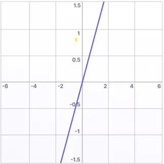
1. Linear Function (Identity Function)
Definition:
The Linear Function (Identity Function) outputs the input as-is, without any transformation.
Mathematical Formula:
f(x) = x

Or with slope:
f(x) = a·x  (where a is a constant)
Graph:
Example:
f(5) = 5
f(-3) = -3
f(0) = 0
f(100) = 100
Characteristics:
| Feature | Description |
|---|---|
| Output Range | (-∞, +∞) |
| Continuity | Continuous |
| Differentiability | Differentiable everywhere |
| Derivative | Constant (usually 1) |
| Linearity | Linear |
When to Use:
- Output layer for regression problems
- When predicting continuous values
- When you don't need non-linearity
Limitation:
- If used in hidden layers, the entire network becomes just a linear model
- No matter how many layers, it's equivalent to a single layer
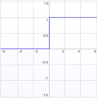
2. Threshold Function (Binary Step Function)
PYQ: Explain threshold function with example (2024, 15 marks)
PYQ: Obtain the output of neuron Y having three inputs x₁=1, x₂=2, x₃=3 and weights w₁=1, w₂=2, w₃=3 by using Threshold activation function. (2022, short answer)
Definition:
The Threshold Function (also called Step Function or Heaviside Function) produces a binary output: either 0 or 1. If the input is greater than or equal to a threshold value, output is 1; otherwise, output is 0.
Mathematical Formula:
f(x) = 1,  if x ≥ θ (threshold)
f(x) = 0,  if x < θ

Note: θ (threshold) is commonly set to 0 when using bias term
Graph:
Example Calculation:
Given:
- Inputs: x₁ = 1, x₂ = 2, x₃ = 3
- Weights: w₁ = 1, w₂ = 2, w₃ = 3
- Threshold: θ = 0
Step 1: Calculate weighted sum
z = (x₁×w₁) + (x₂×w₂) + (x₃×w₃)
z = (1×1) + (2×2) + (3×3)
z = 1 + 4 + 9
z = 14
Step 2: Apply threshold function
Since z = 14 ≥ 0
Output = 1
Characteristics:
| Feature | Description |
|---|---|
| Output Range | {0, 1} (Binary) |
| Continuity | Discontinuous (has a jump) |
| Differentiability | Not differentiable at threshold |
| Use Case | Binary classification |
| Advantage | Simple, easy to understand |
| Disadvantage | Cannot be used in backpropagation |
Real-Life Analogy:
Like a light switch - either ON (1) or OFF (0), nothing in between.
When to Use:
- Simple binary classification problems
- McCulloch-Pitts neuron model
- Perceptron (original version)
- When you need clear yes/no decisions
Limitations:
- No gradient (derivative is 0 everywhere except at threshold where it's undefined)
- Cannot be used in gradient-based learning
- Too rigid for complex problems
3. Signum Function (Sign Function)
Definition:
The Signum Function is similar to the threshold function but outputs -1 or +1 instead of 0 or 1. It's used in bipolar neural networks where outputs need to be bipolar. The function returns +1 if the input is greater than or equal to zero, and -1 if the input is negative.
Mathematical Formula:
f(x) = +1,  if x ≥ 0
f(x) = -1,  if x < 0
Graph:
Output
 +1 |           ┌──────────
    |           |
    |           |
    |-----------|
    |           |
 -1 |           └──────────
    └───────────┴──────────> Input
                0
Example:
Input: x = 5
Output: f(5) = +1

Input: x = -3
Output: f(-3) = -1

Input: x = 0
Output: f(0) = +1
Characteristics:
| Feature | Description |
|---|---|
| Output Range | {-1, +1} (Bipolar) |
| Continuity | Discontinuous |
| Differentiability | Not differentiable at 0 |
| Use Case | Bipolar classification |
Difference from Threshold:
| Aspect | Threshold | Signum |
|---|---|---|
| Output | 0 or 1 | -1 or +1 |
| Type | Unipolar | Bipolar |
| Use | Binary problems | Bipolar problems |
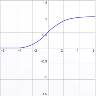
4. Sigmoid Function (Logistic Function)
PYQ: Explain sigmoid function with example (2024, 15 marks)
PYQ: Obtain the output using Sigmoidal activation function (2022, short answer)
Definition:
The Sigmoid Function (also called Logistic Function) produces a smooth S-shaped curve with output values between 0 and 1. It's one of the most popular activation functions in neural networks.
Mathematical Formula:

f(x) = 1 / (1 + e^(-x))

Where:
e = Euler's number (≈ 2.71828)
x = input value
Graph:
At x = -∞, f(x) → 0,
At x = 0, f(x) = 0.5,
At x = ∞, f(x) → 1
Example Calculation:
Given:
- Inputs: x₁ = 1, x₂ = 2, x₃ = 3
- Weights: w₁ = 1, w₂ = 2, w₃ = 3
Step 1: Calculate weighted sum
z = (1×1) + (2×2) + (3×3) = 14
Step 2: Apply sigmoid function
f(14) = 1 / (1 + e^(-14))
f(14) = 1 / (1 + 0.00000083)
f(14) ≈ 0.999999
f(14) ≈ 1
Key Values:
f(0) = 1/(1+e^0) = 1/2 = 0.5
f(1) = 1/(1+e^(-1)) ≈ 0.73
f(2) = 1/(1+e^(-2)) ≈ 0.88
f(-1) = 1/(1+e^1) ≈ 0.27
f(-2) = 1/(1+e^2) ≈ 0.12
f(∞) → 1
f(-∞) → 0
Characteristics:
| Feature | Description |
|---|---|
| Output Range | (0, 1) - Always positive |
| Continuity | Continuous everywhere |
| Differentiability | Differentiable everywhere |
| Derivative | f'(x) = f(x) × (1 - f(x)) |
| Shape | S-shaped curve |
Advantages:
✅ Smooth gradient (good for backpropagation)
✅ Output can be interpreted as probability
✅ Differentiable everywhere
✅ Bounded output (0 to 1)
✅ Non-linear
Disadvantages:
❌ Vanishing gradient problem (for very large/small inputs)
❌ Not zero-centered (output always positive)
❌ Computationally expensive (exponential calculation)
❌ Saturation at extreme values
When to Use:
- Binary classification (output layer)
- When you need probability outputs
- Shallow networks
- When output should be between 0 and 1
Real-Life Analogy:
Like a dimmer switch - gradually increases brightness from 0% to 100%, not just ON/OFF.
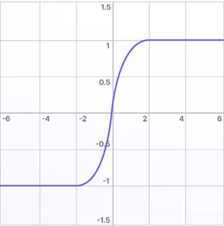
5. Hyperbolic Tangent (tanh) Function
PYQ: Explain tanh function with example (2024, 15 marks)
Definition:
The tanh Function (hyperbolic tangent) is similar to sigmoid but outputs values between -1 and +1. It's zero-centered, making it better than sigmoid in many cases.
Mathematical Formula:

f(x) = tanh(x) = (e^x - e^(-x)) / (e^x + e^(-x))

Alternative form:
f(x) = (e^(2x) - 1) / (e^(2x) + 1)

Or in terms of sigmoid:
f(x) = 2×sigmoid(2x) - 1
Graph:
Example Calculation:
Input: x = 0
tanh(0) = (e^0 - e^0)/(e^0 + e^0) = 0/2 = 0

Input: x = 1
tanh(1) = (e^1 - e^(-1))/(e^1 + e^(-1))
tanh(1) = (2.718 - 0.368)/(2.718 + 0.368)
tanh(1) ≈ 0.76

Input: x = -1
tanh(-1) ≈ -0.76
Key Values:
tanh(0) = 0
tanh(1) ≈ 0.76
tanh(2) ≈ 0.96
tanh(-1) ≈ -0.76
tanh(-2) ≈ -0.96
tanh(∞) → 1
tanh(-∞) → -1
Characteristics:
| Feature | Description |
|---|---|
| Output Range | (-1, +1) - Zero-centered |
| Continuity | Continuous everywhere |
| Differentiability | Differentiable everywhere |
| Derivative | f'(x) = 1 - f(x)² |
| Shape | S-shaped, symmetric |
Comparison: Sigmoid vs Tanh:
| Aspect | Sigmoid | Tanh |
|---|---|---|
| Range | (0, 1) | (-1, 1) |
| Zero-centered | No | Yes |
| Symmetry | Not symmetric | Symmetric around origin |
| Gradient | Smaller | Larger (better) |
| Use | Output layer | Hidden layers |
Advantages:
✅ Zero-centered (better than sigmoid)
✅ Stronger gradients (faster learning)
✅ Symmetric around origin
✅ Differentiable everywhere
Disadvantages:
❌ Still suffers from vanishing gradient
❌ Computationally expensive
❌ Saturation at extreme values
When to Use:
- Hidden layers in neural networks
- When you need zero-centered outputs
- Recurrent neural networks (RNNs)
- When inputs can be negative
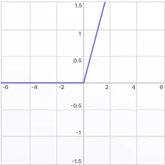
6. ReLU (Rectified Linear Unit)
Definition:
ReLU is the most popular activation function in modern deep learning. It outputs the input directly if positive, otherwise outputs zero.
Mathematical Formula:
f(x) = max(0, x)

Or:
f(x) = x,  if x > 0
f(x) = 0,  if x ≤ 0
Graph:
Example:
f(5) = 5
f(2) = 2
f(0) = 0
f(-3) = 0
f(-10) = 0
Characteristics:
| Feature | Description |
|---|---|
| Output Range | [0, ∞) |
| Continuity | Continuous |
| Differentiability | Not differentiable at 0 |
| Derivative | 1 if x>0, 0 if x<0 |
| Computation | Very fast |
Advantages:
✅ Computationally efficient (just comparison and multiplication)
✅ No vanishing gradient for positive values
✅ Sparse activation (many neurons output 0)
✅ Faster convergence in practice
✅ Most popular in deep learning
Disadvantages:
❌ Dying ReLU problem (neurons can die during training)
❌ Not zero-centered
❌ Unbounded output (can explode)
When to Use:
- Hidden layers in deep networks
- Convolutional Neural Networks (CNNs)
- Default choice for most problems
- When training speed is important
7. Ramp Function
Definition:
The Ramp Function is a combination of linear and threshold functions. It's linear in a range and constant outside.
Mathematical Formula:
f(x) = 0,     if x < 0
f(x) = x,     if 0 ≤ x ≤ 1
f(x) = 1,     if x > 1
Graph:
Output
  1 |        ┌─────────
    |      ╱
    |    ╱
    |  ╱
  0 |─┘
    └────────┴─────────> Input
         0   1
Characteristics:
| Feature | Description |
|---|---|
| Output Range | [0, 1] |
| Continuity | Continuous |
| Linearity | Piecewise linear |
When to Use:
- When you want bounded linear output
- Specific signal processing applications
8. Stochastic Function
Definition:
A Stochastic Function introduces randomness into the activation. The output is probabilistic rather than deterministic.
How it works:
For input x:
- Calculate probability p = sigmoid(x)
- Generate random number r between 0 and 1
- If r < p: output = 1
- Else: output = 0
Characteristics:
| Feature | Description |
|---|---|
| Output | Probabilistic (0 or 1) |
| Deterministic | No (random) |
| Use | Restricted Boltzmann Machines |
When to Use:
- Boltzmann machines
- When you need stochastic behavior
- Specific probabilistic models
2.3 Activation Function Comparison Table
| Function | Range | Continuous | Differentiable | Main Use | Advantage | Disadvantage |
|---|---|---|---|---|---|---|
| Linear | (-∞,∞) | Yes | Yes | Regression output | Simple | No non-linearity |
| Threshold | {0,1} | No | No | Binary classification | Simple | No gradient |
| Signum | {-1,+1} | No | No | Bipolar classification | Simple | No gradient |
| Sigmoid | (0,1) | Yes | Yes | Output layer (binary) | Smooth, probability | Vanishing gradient |
| Tanh | (-1,1) | Yes | Yes | Hidden layers | Zero-centered | Vanishing gradient |
| ReLU | [0,∞) | Yes | Almost | Hidden layers (default) | Fast, no vanishing | Dying ReLU |
| Ramp | [0,1] | Yes | Almost | Special cases | Bounded | Limited use |
| Stochastic | {0,1} | No | No | Probabilistic models | Randomness | Complex |
Section 3: ANN Architecture
3.1 Types of Neural Network Architectures
PYQ: Differentiate between Feedforward and Feedback Networks (2023, 2.5 marks)
Neural networks can be organized in different ways based on how neurons are connected and how information flows through the network. ANN Architecture defines how neurons are organized and connected in a neural network for information processing.

Classification of ANN Architectures:
A. Based on Information Flow:
- Feedforward Network - Information flows in one direction only (input → output)
- Feedback/Recurrent Network - Information can flow in cycles/loops (has memory)
B. Based on Number of Layers:
- Single Layer Network - Only input and output layers (no hidden layer)
- Multilayer Network - Has one or more hidden layers between input and output
C. Based on Connection Pattern:
- Fully Connected Network - Each neuron in one layer is connected to all neurons in the next layer
- Fully Recurrent Network - Every neuron is connected to every other neuron including itself, forming loops within the same layer.
Let's understand each type in detail:
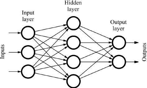
3.2 Feedforward Network
Definition:
A Feedforward Network is a neural network where information flows in only one direction - from input layer through hidden layers to output layer. There are no cycles or loops.
Structure:
Input Layer    Hidden Layer    Output Layer

    x₁ ────────→ h₁ ────────→ y₁
    x₂ ────────→ h₂ ────────→ y₂
    x₃ ────────→ h₃ ────────→ y₃

    Direction: →→→ (One way only)
Characteristics:
- Information flows forward only
- No loops or cycles
- Each layer connects only to the next layer
- Most common type of neural network
- Used for pattern recognition and classification
Types of Feedforward Networks:
1. Single Layer Feedforward Network:
Input → Output (No hidden layer)
2. Multilayer Feedforward Network:
Input → Hidden Layer(s) → Output
Advantages:
- Simple to understand and implement
- Easy to train
- Fast computation
- No memory of past inputs
Disadvantages:
- Cannot handle sequential data
- No memory or context
- Limited to static pattern recognition
Applications:
- Image classification
- Pattern recognition
- Function approximation
- Static data processing
3.3 Feedback Network (Recurrent Network)
Definition:
A Feedback Network (also called Recurrent Network) has connections that form cycles. Information can flow backward or in loops, allowing the network to have memory.
Structure:
Input Layer    Hidden Layer    Output Layer

    x₁ ────────→ h₁ ────────→ y₁
                 ↑ ↓           │
    x₂ ────────→ h₂ ────────→ y₂
                 ↑ ↓           │
    x₃ ────────→ h₃ ────────→ y₃
                 ↑             │
                 └─────────────┘
                   (Feedback Loop)

    Direction: →→→ (Forward) and ←←← (Backward)
Characteristics:
- Information can flow backward
- Has cycles and loops
- Maintains internal state (memory)
- Can process sequential data
- More complex than feedforward
Advantages:
- Has memory of past inputs
- Can handle sequential data
- Good for time-series prediction
- Captures temporal dependencies
Disadvantages:
- Complex to train
- Can be unstable
- Slower computation
- Difficult to optimize
Applications:
- Speech recognition
- Language translation
- Time series prediction
- Video processing
- Text generation
3.4 Single Layer Network
Definition:
A Single Layer Network has only one layer of computational neurons (no hidden layers). Input connects directly to output.
Structure:
Input Layer         Output Layer

    x₁ ─────────────→ y₁
    x₂ ─────────────→ y₂
    x₃ ─────────────→ y₃

    (No hidden layer)
Characteristics:
- Simplest neural network
- Can only solve linearly separable problems
- Limited computational power
- Fast training and testing
Example: Perceptron
Limitations:
- Cannot solve XOR problem
- Cannot learn complex patterns
- Only for simple problems
3.5 Multilayer Network
Definition:
A Multilayer Network has one or more hidden layers between input and output layers. This allows learning complex patterns.
Structure:
Input    Hidden 1    Hidden 2    Output

       ┌──→ h₁₁ ──┬──→ h₂₁ ──┬──→ y₁
       │     ↓    │     ↓    │
  x₁ ──┼──→ h₁₂ ──┼──→ h₂₂ ──┼──→ y₂
  x₂ ──┤     ↓    │     ↓    │
  x₃ ──┘──→ h₁₃ ──┴──→ h₂₃ ──┴──→ y₃

(Each neuron connects to ALL neurons in next layer)
Characteristics:
- Multiple layers of neurons
- Can learn non-linear patterns
- More powerful than single layer
- Requires more training time
Advantages:
- Can solve complex problems
- Learns hierarchical features
- Universal function approximator
- Handles non-linear separability
Disadvantages:
- Requires more data
- Longer training time
- Risk of overfitting
- More parameters to tune
Applications:
- Deep learning
- Image recognition
- Natural language processing
- Complex pattern recognition
3.6 Fully Recurrent Network
Definition:
A Fully Recurrent Network is a network where every neuron is connected to every other neuron, including itself. Maximum connectivity and feedback.
Structure:
       ┌─────────┐
       │   ↓     │
    ┌──→   n₁ ←──┼──┐
    │  │   ↕     │  │
    │  │   ↓     ↓  │
    │  └─→ n₂ ←──┘  │
    │      ↕        │
    │      ↓        │
    └────→ n₃ ←─────┘

    (Every neuron connects to every other neuron including itself)
Characteristics:
- Maximum connectivity
- Every neuron connects to every other
- Complex dynamics
- Can have chaotic behavior
Types:
- Hopfield Network
- Boltzmann Machine
Applications:
- Associative memory
- Optimization problems
- Content-addressable memory
3.7 Architecture Comparison
| Architecture | Connections | Layers | Complexity | Memory | Use Case |
|---|---|---|---|---|---|
| Single Layer Feedforward | Forward only | 1 | Low | No | Simple classification |
| Multilayer Feedforward | Forward only | Multiple | Medium | No | Complex patterns |
| Feedback/Recurrent | Forward + Backward | Multiple | High | Yes | Sequential data |
| Fully Recurrent | All-to-all | Multiple | Very High | Yes | Associative memory |
3.8 Applications of Neural Networks
PYQ: Applications of Neural Network (2024, 2.5 marks)
PYQ: Application of Artificial Neural Network (2023, 15 marks)
Neural networks have revolutionized many fields with their ability to learn complex patterns from data. Here are the major application areas:
1. Computer Vision:
- Image classification (identifying objects in images)
- Face recognition (unlocking phones, security systems)
- Object detection (self-driving cars)
- Medical image analysis (detecting diseases in X-rays, MRIs)
2. Natural Language Processing:
- Machine translation (Google Translate)
- Chatbots (ChatGPT, customer service bots)
- Sentiment analysis (understanding emotions in text)
- Speech recognition (Siri, Alexa)
3. Healthcare:
- Disease diagnosis (cancer detection)
- Drug discovery (finding new medicines)
- Patient monitoring (predicting health issues)
- Medical image analysis (reading X-rays)
4. Finance:
- Stock price prediction
- Fraud detection (credit card fraud)
- Credit scoring (loan approvals)
- Algorithmic trading
5. Autonomous Systems:
- Self-driving cars
- Drones
- Robotics
- Industrial automation
6. Entertainment:
- Recommendation systems (Netflix, YouTube)
- Video game AI
- Music generation
- Art creation
7. Business:
- Customer segmentation
- Sales forecasting
- Marketing optimization
- Demand prediction
Quick Revision Points
Biological Neuron:
- Components: Dendrites (input), Cell body (processing), Axon (output), Synapses (connections)
- Process: Reception → Integration → Decision → Transmission
- Signal: Chemical (neurotransmitters) and Electrical (action potential)
Artificial Neuron Equivalencies:
- Dendrites = Input connections
- Synaptic weights = Connection weights
- Cell body = Summation function
- Threshold = Bias/threshold value
- Axon = Output connection
- Activation = Activation function
Activation Functions:
| Function | Formula | Range | Use |
|---|---|---|---|
| Threshold | 1 if x≥0, else 0 | {0,1} | Binary classification |
| Sigmoid | 1/(1+e^(-x)) | (0,1) | Output layer |
| Tanh | (e^x-e^(-x))/(e^x+e^(-x)) | (-1,1) | Hidden layers |
| ReLU | max(0,x) | [0,∞) | Deep learning (default) |
| Linear | x | (-∞,∞) | Regression |
Network Architectures:
- Feedforward: One-way flow, no loops, static patterns
- Feedback: Loops, memory, sequential data
- Single Layer: No hidden layers, simple problems
- Multilayer: Hidden layers, complex problems
- Fully Recurrent: All-to-all connections, associative memory
Key Formulas:
Neuron Output:
z = Σ(xᵢ × wᵢ) + b
y = f(z)
Sigmoid:
f(x) = 1 / (1 + e^(-x))
f'(x) = f(x) × (1 - f(x))
Tanh:
f(x) = (e^x - e^(-x)) / (e^x + e^(-x))
f'(x) = 1 - f(x)²
Expected Exam Questions
15 Marks Questions:
- Biological neuron structure and signal processing
- Activation functions (threshold, sigmoid, tanh) with examples
- Feedforward vs Feedback networks with architectures
- Applications of neural networks in detail
2.5 Marks Questions:
- Role of dendrites and axons
- Define activation function
- Difference between feedforward and feedback
- Applications of neural networks (list)
- Evolution of neural networks
Numerical Questions:
- Calculate neuron output using threshold function
- Calculate neuron output using sigmoid function
- Apply activation functions to given inputs
These notes were compiled by Deepak Modi
Last updated: December 2025