Syllabus:
McCulloch and Pits Neural Network (MCP Model): Architecture, Solution of AND, OR function using MCP model.
Hebb Model: Architecture, training and testing, Hebb network for AND function.
Perceptron Network: Architecture, training, Testing, single and multi-output model, Perceptron for AND function.
Linear Function: Application of linear model, linear separability, solution of OR function using linear separability model.
PYQ Analysis
High Priority Topics (15 marks questions)
- McCulloch-Pitts Model - (2024: 15 marks, 2023: 15 marks)
- Hebb Model with AND function - (2024: 15 marks, 2023: 15 marks)
- Linear Separability - (2024: 15 marks, 2022: 15 marks)
- Perceptron for OR function - (2022: 15 marks)
Medium Priority Topics (Short answers)
- Linear Separability - 2024 (2.5 marks)
Important Notes:
- Unit 2 is heavily practical with logic function implementations
- Every model requires AND/OR function examples
- Linear separability is a crucial concept
Section 1: McCulloch-Pitts Neural Network (MCP Model)
1.1 Introduction to MCP Model
PYQ: Describe the McCulloch-Pitts (MCP) model in detail. Discuss its architecture, working and the solution for OR functions. (2024, 15 marks)
PYQ: McCulloch Pitts Model (2023, 15 marks)
What is McCulloch-Pitts Model?
The McCulloch-Pitts (MCP) Model is the first mathematical model of a biological neuron, created in 1943 by Warren McCulloch (neuroscientist) and Walter Pitts (mathematician). It's the foundation of all modern neural networks.
Historical Significance:
This model proved that:
- Neurons can perform logical operations (AND, OR, NOT)
- Networks of neurons can compute any logical function
- Brain-like computation is possible with simple units
Key Characteristics:
- Binary inputs (0 or 1)
- Binary output (0 or 1)
- Fixed threshold
- No learning capability (weights are fixed)
- Boolean logic operations
Simple Explanation:
Think of the MCP neuron as a simple decision-maker that:
- Receives multiple yes/no inputs
- Counts how many "yes" inputs it gets
- If the count reaches a threshold, it says "yes" (fires)
- Otherwise, it says "no" (doesn't fire)
1.2 Architecture of MCP Model
Structure:
Inputs (x₁, x₂, ..., xₙ)
    ↓
Weights (all = 1 or -1)
    ↓
Summation (Σ)
    ↓
Threshold (θ)
    ↓
Output (y)
ASCII Diagram:
        x₁ ────→ [w₁=1]
                    ↓
        x₂ ────→ [w₂=1] ──→ Σ ──→ [Threshold θ] ──→ y
                    ↓
        x₃ ────→ [w₃=1]

If Σ(xᵢ × wᵢ) ≥ θ → Output = 1
If Σ(xᵢ × wᵢ) < θ → Output = 0
Visual Diagram:
Figure 2.1: McCulloch-Pitts Neuron Model - Shows inputs (x₁, x₂, ..., xₙ), weights (w₁, w₂, ..., wₙ), summation function (Σ), and threshold activation.
Components:
1. Inputs (x₁, x₂, ..., xₙ):
- Binary values: 0 or 1
- Represent presence (1) or absence (0) of a signal
- Can have multiple inputs
2. Weights (w₁, w₂, ..., wₙ):
- Excitatory weights: +1 (encourage firing)
- Inhibitory weights: -1 (prevent firing)
- Fixed (not learned)
3. Summation Function (Σ):
- Adds up all weighted inputs
- Formula: Σ = (x₁×w₁) + (x₂×w₂) + ... + (xₙ×wₙ)
4. Threshold (θ):
- Fixed value
- Decision boundary
- Determines when neuron fires
5. Output (y):
- Binary: 0 or 1
- 1 if sum ≥ threshold
- 0 if sum < threshold
1.3 Working of MCP Model
Step-by-Step Process:
Step 1: Receive Inputs
- Get binary inputs (0 or 1) from other neurons or external sources
Step 2: Apply Weights
- Multiply each input by its weight
- Excitatory: multiply by +1
- Inhibitory: multiply by -1
Step 3: Calculate Sum
- Add all weighted inputs
- Σ = Σ(xᵢ × wᵢ)
Step 4: Compare with Threshold
- If Σ ≥ θ → Output = 1 (neuron fires)
- If Σ < θ → Output = 0 (neuron doesn't fire)
Mathematical Representation:
y = 1,  if Σ(xᵢ × wᵢ) ≥ θ
y = 0,  if Σ(xᵢ × wᵢ) < θ

Or using step function:
y = step(Σ(xᵢ × wᵢ) - θ)
1.4 MCP Model for AND Function
PYQ: Solution of AND function using MCP model (2024, 15 marks)
AND function can be implemented using MCP model by setting the weights to 1 and the threshold to 2.
AND Function Truth Table:
| x₁ | x₂ | y (x₁ AND x₂) |
|---|---|---|
| 0 | 0 | 0 |
| 0 | 1 | 0 |
| 1 | 0 | 0 |
| 1 | 1 | 1 |
Logic: Output is 1 only when BOTH inputs are 1.
MCP Design for AND:
x₁ ────→ [w₁ = 1]
                  ↘
                   Σ ──→ [θ = 2] ──→ y
                  ↗
x₂ ────→ [w₂ = 1]
Parameters:
- Weights: w₁ = 1, w₂ = 1 (both excitatory)
- Threshold: θ = 2
Why θ = 2?
- For output to be 1, we need BOTH inputs to be 1
- Sum = 1×1 + 1×1 = 2
- So threshold should be 2
Verification:
Case 1: x₁ = 0, x₂ = 0
Σ = (0×1) + (0×1) = 0
Since 0 < 2 → y = 0 ✓
Case 2: x₁ = 0, x₂ = 1
Σ = (0×1) + (1×1) = 1
Since 1 < 2 → y = 0 ✓
Case 3: x₁ = 1, x₂ = 0
Σ = (1×1) + (0×1) = 1
Since 1 < 2 → y = 0 ✓
Case 4: x₁ = 1, x₂ = 1
Σ = (1×1) + (1×1) = 2
Since 2 ≥ 2 → y = 1 ✓
Complete Solution Table:
| x₁ | x₂ | w₁×x₁ | w₂×x₂ | Σ | θ | y |
|---|---|---|---|---|---|---|
| 0 | 0 | 0 | 0 | 0 | 2 | 0 |
| 0 | 1 | 0 | 1 | 1 | 2 | 0 |
| 1 | 0 | 1 | 0 | 1 | 2 | 0 |
| 1 | 1 | 1 | 1 | 2 | 2 | 1 |
1.5 MCP Model for OR Function
PYQ: Solution of OR function using MCP model (2024, 15 marks)
OR function can be implemented using MCP model by setting the weights to 1 and the threshold to 1.
OR Function Truth Table:
| x₁ | x₂ | y (x₁ OR x₂) |
|---|---|---|
| 0 | 0 | 0 |
| 0 | 1 | 1 |
| 1 | 0 | 1 |
| 1 | 1 | 1 |
Logic: Output is 1 when AT LEAST ONE input is 1.
MCP Design for OR:
x₁ ────→ [w₁ = 1]
                  ↘
                   Σ ──→ [θ = 1] ──→ y
                  ↗
x₂ ────→ [w₂ = 1]
Parameters:
- Weights: w₁ = 1, w₂ = 1 (both excitatory)
- Threshold: θ = 1
Why θ = 1?
- For output to be 1, we need AT LEAST ONE input to be 1
- Minimum sum when one input is 1: 1×1 = 1
- So threshold should be 1
Verification:
Case 1: x₁ = 0, x₂ = 0
Σ = (0×1) + (0×1) = 0
Since 0 < 1 → y = 0 ✓
Case 2: x₁ = 0, x₂ = 1
Σ = (0×1) + (1×1) = 1
Since 1 ≥ 1 → y = 1 ✓
Case 3: x₁ = 1, x₂ = 0
Σ = (1×1) + (0×1) = 1
Since 1 ≥ 1 → y = 1 ✓
Case 4: x₁ = 1, x₂ = 1
Σ = (1×1) + (1×1) = 2
Since 2 ≥ 1 → y = 1 ✓
Complete Solution Table:
| x₁ | x₂ | w₁×x₁ | w₂×x₂ | Σ | θ | y |
|---|---|---|---|---|---|---|
| 0 | 0 | 0 | 0 | 0 | 1 | 0 |
| 0 | 1 | 0 | 1 | 1 | 1 | 1 |
| 1 | 0 | 1 | 0 | 1 | 1 | 1 |
| 1 | 1 | 1 | 1 | 2 | 1 | 1 |
1.6 MCP Model for NOT Function
NOT function can be implemented using MCP model by setting the weight to -1 and the threshold to 0.
NOT Function Truth Table:
| x | y (NOT x) |
|---|---|
| 0 | 1 |
| 1 | 0 |
Logic: Output is opposite of input.
MCP Design for NOT:
x ────→ [w = -1] ──→ Σ ──→ [θ = 0] ──→ y
Parameters:
- Weight: w = -1 (inhibitory)
- Threshold: θ = 0
Verification:
Case 1: x = 0
Σ = 0×(-1) = 0
Since 0 ≥ 0 → y = 1 ✓
Case 2: x = 1
Σ = 1×(-1) = -1
Since -1 < 0 → y = 0 ✓
Complete Solution Table:
| x | w×x | Σ | θ | y |
|---|---|---|---|---|
| 0 | 0 | 0 | 0 | 1 |
| 1 | -1 | -1 | 0 | 0 |
1.7 Characteristics of MCP Model
Advantages:
✅ First mathematical model of a neuron
✅ Simple and easy to understand
✅ Can implement basic logic functions
✅ Foundation for modern neural networks
✅ Proved that neurons can compute
Disadvantages:
❌ No learning capability (weights are fixed)
❌ Only binary inputs and outputs
❌ Cannot solve non-linearly separable problems (XOR)
❌ Weights must be manually set
❌ Limited to simple Boolean functions
Limitations:
- No Learning: Weights are predetermined, not learned from data
- Binary Only: Cannot handle continuous values
- XOR Problem: Cannot solve XOR function (non-linearly separable)
- Manual Design: Requires human to set weights and threshold
Section 2: Hebb Model
2.1 Introduction to Hebb Model
PYQ: Explain Hebbian Model and implement logic 'AND' function using Hebb Network. (2024, 15 marks)
PYQ: Explain Hebbian Model and implement logic 'AND' function using Hebb Network. (2023, 15 marks)
What is Hebb Model?
The Hebb Model (1949) is a neural network that can learn from examples. It was proposed by Donald Hebb, a Canadian psychologist, based on how biological neurons learn.
Hebb's Learning Rule:
"Cells that fire together, wire together"
This means:
- When two neurons are active at the same time, the connection between them gets stronger
- When they're not active together, the connection weakens or stays the same
Key Innovation:
Unlike MCP model (fixed weights), Hebb model can adjust weights based on training data. This was the first learning algorithm for neural networks!
Characteristics:
- Can learn from examples
- Adjusts weights automatically
- Simple learning rule
- Supervised learning
- Used for pattern association
2.2 Architecture of Hebb Model
Structure:
Training Phase:
    Inputs (x₁, x₂, ..., xₙ)
        ↓
    Initial Weights (w₁=0, w₂=0, ..., wₙ=0)
        ↓
    Weight Update (Hebbian Learning)
        ↓
    Final Weights

Testing Phase:
    New Inputs
        ↓
    Learned Weights
        ↓
    Summation
        ↓
    Activation Function
        ↓
    Output
Components:
- Input Layer: Receives input patterns
- Weights: Initially zero, updated during training
- Bias: Additional adjustable parameter
- Activation Function: Usually step function or bipolar step
- Output: Predicted result
2.3 Hebbian Learning Algorithm
Training Algorithm:
Step 1: Initialize
    Set all weights to 0: w₁ = w₂ = ... = wₙ = 0
    Set bias to 0: b = 0

Step 2: For each training pattern (x, y):
    Step 2a: Calculate weight updates
        Δwᵢ = xᵢ × y  (for each input i)
        Δb = y

    Step 2b: Update weights
        wᵢ(new) = wᵢ(old) + Δwᵢ
        b(new) = b(old) + Δb

Step 3: Repeat Step 2 for all training patterns

Step 4: Final weights are learned
Mathematical Formula:
Weight Update:
wᵢ(new) = wᵢ(old) + (xᵢ × y)

Bias Update:
b(new) = b(old) + y

Where:
- xᵢ = input value
- y = desired output (target)
- wᵢ = weight for input i
- b = bias
Testing Algorithm:
Step 1: For new input pattern x:
    Calculate: y_in = Σ(xᵢ × wᵢ) + b

Step 2: Apply activation function:
    If y_in ≥ 0: y = +1
    If y_in < 0: y = -1  (for bipolar)

    Or:
    If y_in ≥ 0: y = 1
    If y_in < 0: y = 0   (for binary)

Step 3: Output y

Where:
- y_in = input to activation function
- y = output of activation function
2.4 Hebb Network for AND Function
PYQ: Implement logic 'AND' function using Hebb Network (2024, 2023, 15 marks)
Problem Statement:
Design a Hebb network to implement the AND function using bipolar inputs and outputs.
AND Function Truth Table (Bipolar):
| x₁ | x₂ | y (x₁ AND x₂) |
|---|---|---|
| -1 | -1 | -1 |
| -1 | +1 | -1 |
| +1 | -1 | -1 |
| +1 | +1 | +1 |
Note: Using bipolar (-1, +1) instead of binary (0, 1) for better learning.
Solution:
Step 1: Initialize Weights and Bias
w₁ = 0
w₂ = 0
b = 0
Step 2: Training with Pattern 1 (x₁=-1, x₂=-1, y=-1)
Calculate weight updates:
Δw₁ = x₁ × y = (-1) × (-1) = 1
Δw₂ = x₂ × y = (-1) × (-1) = 1
Δb = y = -1

Update weights:
w₁ = 0 + 1 = 1
w₂ = 0 + 1 = 1
b = 0 + (-1) = -1
Step 3: Training with Pattern 2 (x₁=-1, x₂=+1, y=-1)
Calculate weight updates:
Δw₁ = x₁ × y = (-1) × (-1) = 1
Δw₂ = x₂ × y = (+1) × (-1) = -1
Δb = y = -1

Update weights:
w₁ = 1 + 1 = 2
w₂ = 1 + (-1) = 0
b = -1 + (-1) = -2
Step 4: Training with Pattern 3 (x₁=+1, x₂=-1, y=-1)
Calculate weight updates:
Δw₁ = x₁ × y = (+1) × (-1) = -1
Δw₂ = x₂ × y = (-1) × (-1) = 1
Δb = y = -1

Update weights:
w₁ = 2 + (-1) = 1
w₂ = 0 + 1 = 1
b = -2 + (-1) = -3
Step 5: Training with Pattern 4 (x₁=+1, x₂=+1, y=+1)
Calculate weight updates:
Δw₁ = x₁ × y = (+1) × (+1) = 1
Δw₂ = x₂ × y = (+1) × (+1) = 1
Δb = y = +1

Update weights:
w₁ = 1 + 1 = 2
w₂ = 1 + 1 = 2
b = -3 + 1 = -2
Final Learned Weights:
w₁ = 2
w₂ = 2
b = -2
Training Summary Table:
| Pattern | x₁ | x₂ | y | Δw₁ | Δw₂ | Δb | w₁ | w₂ | b |
|---|---|---|---|---|---|---|---|---|---|
| Initial | - | - | - | - | - | - | 0 | 0 | 0 |
| 1 | -1 | -1 | -1 | 1 | 1 | -1 | 1 | 1 | -1 |
| 2 | -1 | +1 | -1 | 1 | -1 | -1 | 2 | 0 | -2 |
| 3 | +1 | -1 | -1 | -1 | 1 | -1 | 1 | 1 | -3 |
| 4 | +1 | +1 | +1 | 1 | 1 | +1 | 2 | 2 | -2 |
Step 6: Testing
Now let's test with all input patterns:
Test 1: x₁ = -1, x₂ = -1
y_in = (x₁ × w₁) + (x₂ × w₂) + b
y_in = (-1 × 2) + (-1 × 2) + (-2)
y_in = -2 + (-2) + (-2)
y_in = -6

Since y_in < 0 → y = -1 ✓ (Correct!)
Test 2: x₁ = -1, x₂ = +1
y_in = (-1 × 2) + (+1 × 2) + (-2)
y_in = -2 + 2 + (-2)
y_in = -2

Since y_in < 0 → y = -1 ✓ (Correct!)
Test 3: x₁ = +1, x₂ = -1
y_in = (+1 × 2) + (-1 × 2) + (-2)
y_in = 2 + (-2) + (-2)
y_in = -2

Since y_in < 0 → y = -1 ✓ (Correct!)
Test 4: x₁ = +1, x₂ = +1
y_in = (+1 × 2) + (+1 × 2) + (-2)
y_in = 2 + 2 + (-2)
y_in = 2

Since y_in > 0 → y = +1 ✓ (Correct!)
Testing Results Table:
| x₁ | x₂ | w₁×x₁ | w₂×x₂ | b | y_in | y (output) | Expected | Result |
|---|---|---|---|---|---|---|---|---|
| -1 | -1 | -2 | -2 | -2 | -6 | -1 | -1 | ✓ |
| -1 | +1 | -2 | +2 | -2 | -2 | -1 | -1 | ✓ |
| +1 | -1 | +2 | -2 | -2 | -2 | -1 | -1 | ✓ |
| +1 | +1 | +2 | +2 | -2 | +2 | +1 | +1 | ✓ |
Conclusion: The Hebb network successfully learned the AND function! All test cases pass.
2.5 Characteristics of Hebb Model
Advantages:
✅ First learning algorithm for neural networks
✅ Simple and intuitive
✅ Biologically inspired
✅ Can learn from examples
✅ Automatic weight adjustment
Disadvantages:
❌ Weights can grow unbounded
❌ No mechanism to unlearn
❌ Limited to linearly separable problems
❌ Sensitive to training order
❌ May not converge for all problems
When to Use:
- Simple pattern association
- Linearly separable problems
- When biological plausibility is important
- Educational purposes
Section 3: Perceptron Network
3.1 Introduction to Perceptron
PYQ: What is perceptron? Also realize it for OR function for bipolar data. (2022, 15 marks)
What is Perceptron?
The Perceptron (1958) was invented by Frank Rosenblatt. It's an improved version of the MCP model with a better learning algorithm. It was the first neural network that could actually learn to classify patterns automatically.
Key Innovation:
- Perceptron Learning Rule: Better than Hebbian learning
- Guaranteed Convergence: For linearly separable problems
- Error Correction: Adjusts weights only when mistakes are made
Historical Significance:
- First hardware implementation of a neural network (Mark I Perceptron)
- Could learn to recognize patterns from images
- Sparked the first wave of AI enthusiasm
- Foundation for modern deep learning
Characteristics:
- Single layer feedforward network
- Supervised learning
- Binary or bipolar outputs
- Iterative weight adjustment
- Convergence theorem (for linearly separable data)
3.2 Architecture of Perceptron
Structure:
Input Layer        Perceptron        Output

    x₁ ──[w₁]──┐
               │
    x₂ ──[w₂]──┤
               ├──→ Σ ──→ f(.) ──→ y
    x₃ ──[w₃]──┤    ↑
               │  [bias]
    xₙ ──[wₙ]───┘
Visual Diagram:
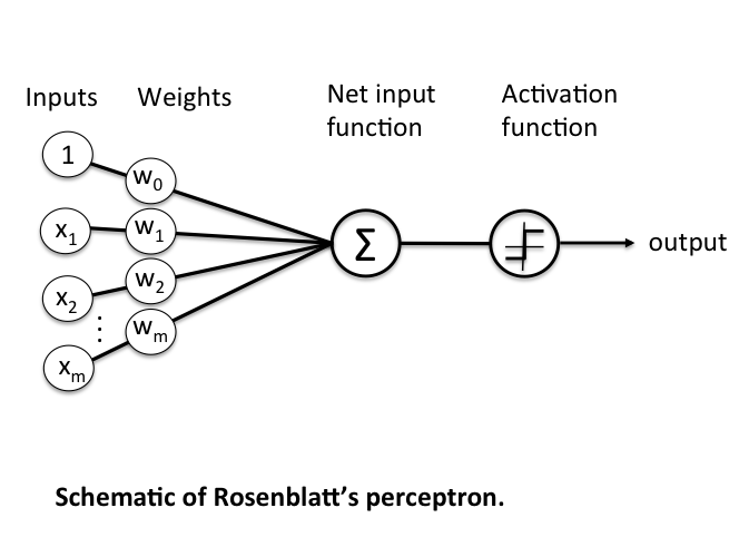
Figure 2.2: Perceptron Architecture - Shows input layer with weighted connections, summation unit, activation function, and output.
Components:
- Input Layer: x₁, x₂, ..., xₙ (features)
- Weights: w₁, w₂, ..., wₙ (adjustable)
- Bias: b (threshold adjustment)
- Summation: Σ(xᵢ × wᵢ) + b
- Activation Function: Step function or bipolar step
- Output: y (classification result)
Types of Perceptron:
1. Single Output Perceptron:
- One output neuron
- Binary classification (2 classes)
- Example: AND, OR, NOT
2. Multi-Output Perceptron:
- Multiple output neurons
- Multi-class classification
- Each output for one class
3.3 Perceptron Learning Algorithm
Training Algorithm:
Step 1: Initialize
    Set weights to small random values or 0
    Set learning rate α (typically 0.1 to 1)
    Set bias b = 0

Step 2: For each training pattern (x, t):
    Step 2a: Calculate output
        y_in = Σ(xᵢ × wᵢ) + b
        y = f(y_in)  [Apply activation function]

    Step 2b: Calculate error
        error = t - y
        (t = target/desired output)

    Step 2c: Update weights (only if error ≠ 0)
        If error ≠ 0:
            wᵢ(new) = wᵢ(old) + α × error × xᵢ
            b(new) = b(old) + α × error

Step 3: Repeat Step 2 until:
    - All patterns classified correctly, OR
    - Maximum epochs (dataset passes) reached

Step 4: Return learned weights
Weight Update Rule:
Δwᵢ = α × (t - y) × xᵢ

Where:
- α = learning rate (controls step size)
- t = target output (desired)
- y = actual output (predicted)
- xᵢ = input value
Key Difference from Hebb:
| Aspect | Hebb Rule | Perceptron Rule |
|---|---|---|
| Update | Always | Only on error |
| Formula | Δw = x × y | Δw = α × (t-y) × x |
| Error Correction | No | Yes |
| Convergence | Not guaranteed | Guaranteed (if linearly separable) |
3.4 Perceptron for AND Function
Problem: Implement AND function using Perceptron with bipolar inputs.
AND Function Truth Table (Bipolar):
| x₁ | x₂ | t (target) |
|---|---|---|
| -1 | -1 | -1 |
| -1 | +1 | -1 |
| +1 | -1 | -1 |
| +1 | +1 | +1 |
Solution:
Initial Setup:
w₁ = 0, w₂ = 0, b = 0
α = 1 (learning rate)
Activation: bipolar step function
Epoch 1:
Pattern 1: x₁=-1, x₂=-1, t=-1
y_in = (-1×0) + (-1×0) + 0 = 0
y = sign(0) = +1  (assuming sign(0) = +1)
error = t - y = -1 - (+1) = -2

Update weights:
w₁ = 0 + 1×(-2)×(-1) = 2
w₂ = 0 + 1×(-2)×(-1) = 2
b = 0 + 1×(-2) = -2
Pattern 2: x₁=-1, x₂=+1, t=-1
y_in = (-1×2) + (+1×2) + (-2) = -2
y = sign(-2) = -1
error = -1 - (-1) = 0

No update (error = 0)
w₁ = 2, w₂ = 2, b = -2
Pattern 3: x₁=+1, x₂=-1, t=-1
y_in = (+1×2) + (-1×2) + (-2) = -2
y = sign(-2) = -1
error = -1 - (-1) = 0

No update
w₁ = 2, w₂ = 2, b = -2
Pattern 4: x₁=+1, x₂=+1, t=+1
y_in = (+1×2) + (+1×2) + (-2) = 2
y = sign(2) = +1
error = +1 - (+1) = 0

No update
w₁ = 2, w₂ = 2, b = -2
Final Weights: w₁=2, w₂=2, b=-2
Testing: (Same as Hebb model testing - all patterns correctly classified)
3.5 Perceptron for OR Function (Bipolar)
PYQ: Realize Perceptron for OR function for bipolar data (2022, 15 marks)
OR Function Truth Table (Bipolar):
| x₁ | x₂ | t (target) |
|---|---|---|
| -1 | -1 | -1 |
| -1 | +1 | +1 |
| +1 | -1 | +1 |
| +1 | +1 | +1 |
Solution:
Initial Setup:
w₁ = 0, w₂ = 0, b = 0
α = 1
Epoch 1:
Pattern 1: x₁=-1, x₂=-1, t=-1
y_in = 0
y = +1
error = -1 - (+1) = -2

Update:
w₁ = 0 + 1×(-2)×(-1) = 2
w₂ = 0 + 1×(-2)×(-1) = 2
b = 0 + 1×(-2) = -2
Pattern 2: x₁=-1, x₂=+1, t=+1
y_in = (-1×2) + (+1×2) + (-2) = -2
y = -1
error = +1 - (-1) = 2

Update:
w₁ = 2 + 1×(2)×(-1) = 0
w₂ = 2 + 1×(2)×(+1) = 4
b = -2 + 1×(2) = 0
Pattern 3: x₁=+1, x₂=-1, t=+1
y_in = (+1×0) + (-1×4) + 0 = -4
y = -1
error = +1 - (-1) = 2

Update:
w₁ = 0 + 1×(2)×(+1) = 2
w₂ = 4 + 1×(2)×(-1) = 2
b = 0 + 1×(2) = 2
Pattern 4: x₁=+1, x₂=+1, t=+1
y_in = (+1×2) + (+1×2) + 2 = 6
y = +1
error = +1 - (+1) = 0

No update
Final: w₁ = 2, w₂ = 2, b = 2
Testing:
| x₁ | x₂ | y_in | y | Expected | Result |
|---|---|---|---|---|---|
| -1 | -1 | -2 | -1 | -1 | ✓ |
| -1 | +1 | 2 | +1 | +1 | ✓ |
| +1 | -1 | 2 | +1 | +1 | ✓ |
| +1 | +1 | 6 | +1 | +1 | ✓ |
Success! The perceptron learned the OR function.
3.6 Characteristics of Perceptron
Advantages:
✅ Guaranteed convergence for linearly separable problems
✅ Error-correction learning (only updates on mistakes)
✅ Simple and efficient
✅ First practical learning algorithm
✅ Foundation for modern neural networks
Disadvantages:
❌ Cannot solve non-linearly separable problems (XOR)
❌ Single layer limitation
❌ No convergence guarantee for non-separable data
❌ Sensitive to learning rate
❌ May oscillate if not linearly separable
Perceptron Convergence Theorem:
If the training data is linearly separable, the perceptron learning algorithm will converge in a finite number of steps.
Section 4: Linear Separability
4.1 What is Linear Separability?
PYQ: Illustrate the concept of linear separability with the solution of the OR function. (2024, 15 marks)
PYQ: Explain Linear Separability Concept by taking a suitable example, also classify the output of OR function using it. (2022, 15 marks)
PYQ: Linear Separability (2024, 2.5 marks)
Definition:
Linear Separability means that two classes of data points can be separated by a straight line (in 2D), a plane (in 3D), or a hyperplane (in higher dimensions).
Simple Explanation:
Imagine you have red dots and green dots on a paper. If you can draw a straight line that puts all red dots on one side and all green dots on the other side, then the data is linearly separable. Otherwise, it is non-linearly separable.
Mathematical Definition:
A dataset is linearly separable if there exists a hyperplane:
w₁x₁ + w₂x₂ + ... + wₙxₙ + b = 0
such that:
- For class +1: w₁x₁ + w₂x₂ + ... + wₙxₙ + b > 0
- For class -1: w₁x₁ + w₂x₂ + ... + wₙxₙ + b < 0
4.2 Geometric Interpretation
A decision boundary separates the two classes. In 2D space, this boundary is a straight line; in 3D, it's a plane; and in higher dimensions, it's called a hyperplane.
2D Example:
      x₂
       ↑
    +1 |    ○         ○  (Class +1)
       |
       |  ╱ Decision Boundary
     0 | ╱
       |╱
   -1  |●         ●      (Class -1)
       └──────────────→ x₁
      -1    0    +1
Decision Boundary Equation:
w₁x₁ + w₂x₂ + b = 0

This is a straight line in 2D
Classification Rule:
Bipolar Representation:
If w₁x₁ + w₂x₂ + b > 0 → Class +1 (●)
If w₁x₁ + w₂x₂ + b < 0 → Class -1 (○)

OR

Binary Representation:
If w₁x₁ + w₂x₂ + b ≥ 0 → Class 1 (●)
If w₁x₁ + w₂x₂ + b < 0 → Class 0 (○)
Note: We will be using bipolar representation (+1, -1) instead of binary (0, 1) because the Perceptron uses the Signum activation function which outputs -1 or +1, and bipolar values provide better mathematical properties for weight updates during learning. However, binary (0, 1) representation can also be used with appropriate activation functions like the threshold function.
4.3 Linear Separability of Logic Functions
AND Function (Linearly Separable):
AND output is +1 when both inputs are +1, otherwise -1.
Truth Table:
x₁  x₂  | y
-1  -1  | -1  ●
-1  +1  | -1  ●
+1  -1  | -1  ●
+1  +1  | +1  ○

Plot:
      x₂
       ↑
    +1 |    ●         ○
       |       ╱
       |     ╱
     0 |   ╱
       | ╱
   -1  |●         ●
       └──────────────→ x₁
      -1    0    +1

Decision Line: x₁ + x₂ = 1
Can separate! ✓
OR Function (Linearly Separable):
OR output is +1 when at least one input is +1, otherwise -1.
Truth Table:
x₁  x₂  | y
-1  -1  | -1  ●
-1  +1  | +1  ○
+1  -1  | +1  ○
+1  +1  | +1  ○

Plot:
      x₂
       ↑
    +1 |    ○         ○
       |   ╱
       | ╱
     0 |╱
       |
   -1  |●
       └──────────────→ x₁
      -1    0    +1

Decision Line: x₁ + x₂ = 0
Can separate! ✓
XOR Function (NOT Linearly Separable):
XOR output is +1 when the inputs are different, otherwise -1.
Truth Table:
x₁  x₂  | y
-1  -1  | -1  ●
-1  +1  | +1  ○
+1  -1  | +1  ○
+1  +1  | -1  ●

Plot:
      x₂
       ↑
    +1 |    ○         ●
       |
       |
     0 |
       |
   -1  |●         ○
       └──────────────→ x₁
      -1    0    +1

Cannot draw a single line to separate! ✗
This is why single-layer perceptron fails on XOR!
Visual Diagram:
This is for binary (0, 1) representation.
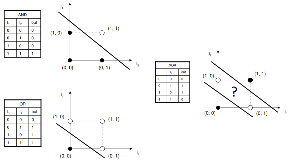
This is for bipolar (-1, +1) representation.

Figure 2.3: Linear Separability - AND and OR functions are linearly separable (can be separated by a line), but XOR is not (requires a curved boundary or multiple layers).
4.4 Solution of OR Function using Linear Separability
PYQ: Solution of OR function using linear separability model (2024, 2022, 15 marks)
Step 1: Plot the Data Points
OR Function (Bipolar):
(-1, -1) → -1  [Point A: Class -1]
(-1, +1) → +1  [Point B: Class +1]
(+1, -1) → +1  [Point C: Class +1]
(+1, +1) → +1  [Point D: Class +1]

Plot:
      x₂
       ↑
    +1 | B(○)      D(○)
       |
       |
     0 |
       |
   -1  | A(●)      C(○)
       └────────────────→ x₁
      -1    0     +1
Step 2: Find Decision Boundary
We need a line that separates:
- Class -1 (only point A)
- Class +1 (points B, C, D)
Try the line: x₁ + x₂ = 0
For point A (-1, -1):
x₁ + x₂ = -1 + (-1) = -2 < 0 ✓ (Class -1)

For point B (-1, +1):
x₁ + x₂ = -1 + 1 = 0 ≥ 0 ✓ (Class +1)

For point C (+1, -1):
x₁ + x₂ = 1 + (-1) = 0 ≥ 0 ✓ (Class +1)

For point D (+1, +1):
x₁ + x₂ = 1 + 1 = 2 > 0 ✓ (Class +1)
Decision Boundary Found!
Equation: x₁ + x₂ = 0
Or: w₁x₁ + w₂x₂ + b = 0

Where: w₁ = 1, w₂ = 1, b = 0
Step 3: Classification Rule
If x₁ + x₂ ≥ 0 → Output = +1
If x₁ + x₂ < 0 → Output = -1
Step 4: Verification
| x₁ | x₂ | x₁+x₂ | Output | Expected | Result |
|---|---|---|---|---|---|
| -1 | -1 | -2 | -1 | -1 | ✓ |
| -1 | +1 | 0 | +1 | +1 | ✓ |
| +1 | -1 | 0 | +1 | +1 | ✓ |
| +1 | +1 | 2 | +1 | +1 | ✓ |
Conclusion: OR function is linearly separable with decision boundary x₁ + x₂ = 0.
4.5 Why XOR is Not Linearly Separable
XOR Truth Table:
| x₁ | x₂ | y |
|---|---|---|
| 0 | 0 | 0 |
| 0 | 1 | 1 |
| 1 | 0 | 1 |
| 1 | 1 | 0 |
Problem:
Plot:
      x₂
       ↑
     1 |    ○         ●
       |
       |
     0 |●         ○
       └──────────────→ x₁
       0    1

○ = Class 1 (output = 1)
● = Class 0 (output = 0)

No single straight line can separate these!
Why Single-Layer Networks Fail:
- Single-layer perceptron can only learn linearly separable functions
- XOR requires a curved or multiple decision boundaries
- This limitation led to the "AI Winter" in the 1970s
- Solution: Multi-layer networks (covered in Unit 3)
4.6 Testing for Linear Separability
Methods to Check:
1. Visual Method (2D):
- Plot the points
- Try to draw a straight line
- If possible → linearly separable
2. Analytical Method:
- Try to find weights w and bias b
- Such that all points are correctly classified
- If found → linearly separable
3. Computational Method:
- Train a perceptron
- If it converges → linearly separable
- If it doesn't converge → not linearly separable
Comparison of Models
Summary Table
| Feature | MCP Model | Hebb Model | Perceptron |
|---|---|---|---|
| Year | 1943 | 1949 | 1958 |
| Learning | No | Yes | Yes |
| Weight Update | Fixed | Always | On error only |
| Convergence | N/A | Not guaranteed | Guaranteed (if separable) |
| Complexity | Simplest | Simple | Moderate |
| Biological | Yes | Very yes | Less |
| Practical Use | Limited | Limited | Historical |
Which to Use When?
MCP Model:
- Understanding basic concepts
- Simple Boolean logic
- Educational purposes
- When weights are known
Hebb Model:
- Biologically plausible learning
- Pattern association
- Simple problems
- Educational purposes
Perceptron:
- Binary classification
- Linearly separable problems
- When guaranteed convergence needed
- Foundation for understanding deep learning
Quick Revision Points
MCP Model:
- First mathematical neuron model (1943)
- Fixed weights (no learning)
- Binary inputs/outputs
- Can implement AND, OR, NOT
- Cannot solve XOR
Hebb Model:
- First learning algorithm (1949)
- "Cells that fire together, wire together"
- Weight update: Δw = x × y
- Always updates weights
- Not guaranteed to converge
Perceptron:
- Improved learning algorithm (1958)
- Weight update: Δw = α × (t-y) × x
- Updates only on errors
- Guaranteed convergence (if linearly separable)
- Cannot solve XOR (single layer)
Linear Separability:
- Data can be separated by a straight line/plane
- AND, OR → linearly separable ✓
- XOR → not linearly separable ✗
- Single-layer networks limited to linearly separable problems
- Multi-layer networks can solve non-linearly separable problems
Key Formulas:
MCP Output:
y = 1 if Σ(xᵢwᵢ) ≥ θ, else 0
Hebb Weight Update:
wᵢ(new) = wᵢ(old) + (xᵢ × y)
Perceptron Weight Update:
wᵢ(new) = wᵢ(old) + α × (t - y) × xᵢ
Decision Boundary:
w₁x₁ + w₂x₂ + ... + wₙxₙ + b = 0
Expected Exam Questions
15 Marks Questions:
- MCP model architecture and AND/OR function implementation
- Hebb model and implement AND function with complete training
- Perceptron for OR function (bipolar) with training and testing
- Linear separability concept with OR function solution
- Compare MCP, Hebb, and Perceptron models
2.5 Marks Questions:
- Define linear separability
- MCP model architecture
- Hebbian learning rule
- Perceptron convergence theorem
- Why XOR is not linearly separable
Numerical Questions:
- Train Hebb network for AND function (complete steps)
- Train Perceptron for OR function (show all epochs)
- Find decision boundary for given data points
- Verify linear separability of a logic function
These notes were compiled by Deepak Modi
Last updated: December 2025