Syllabus:
Learning: Supervised, Unsupervised, reinforcement learning, Gradient Descent algorithm, generalized delta learning rule, Hebbian learning, Competitive learning.
Back Propagation Network: Architecture, training and testing.
PYQ Analysis
High Priority Topics (15 marks questions)
- Backpropagation Network - (2024: 15 marks, 2023: 2.5 marks)
- Gradient Descent Algorithm - (2023: 15 marks, 2022: 15 marks)
- Generalized Delta Rule - (2023: 15 marks, 2022: 15 marks)
- Competitive Learning - (2024: 15 marks, 2022: short)
- Learning Types - (2022: 15 marks)
Medium Priority Topics (Short answers)
- Supervised Learning - 2024 (2.5 marks)
- Unsupervised Learning - 2023 (2.5 marks)
- Reinforcement Learning - 2023 (2.5 marks)
- Backpropagation Network - 2023 (2.5 marks)
- Generalized Delta Learning Rule - 2024 (2.5 marks)
- Separability limitations in unsupervised Learning - 2023 (2.5 marks)
Important Notes:
- Unit 3 is algorithm-heavy with derivations
- Learning types are fundamental concepts
- Backpropagation is the most important topic
- Gradient descent requires mathematical understanding
Section 1: Types of Learning
1.1 What is Learning in Neural Networks?
PYQ: What is Learning? Explain its different types. (2022, 15 marks)
Definition:
Learning in neural networks is the process of adjusting the connection weights (and biases) based on training data so that the network can make accurate predictions or classifications on new, unseen data.
Simple Explanation:
Think of learning like a student studying for an exam:
- Training data = Practice problems
- Learning = Understanding patterns and rules
- Testing = Solving new problems in the exam
- Weights = Knowledge gained
Why is Learning Important?
- Allows networks to improve from experience
- Enables automatic feature extraction
- Adapts to new patterns
- Reduces manual programming
- Makes AI possible
Learning Process:
Input Data → Neural Network → Output
                ↓
           Compare with
         Expected Output
                ↓
          Calculate Error
                ↓
         Adjust Weights
                ↓
         Repeat Until
      Error is Minimized
1.2 Supervised Learning
PYQ: Supervised Learning (2024, 2.5 marks)
Definition:
Supervised Learning is a type of learning where the network is trained using labeled data. For each input, we know the correct output (target/label), and the network learns to map inputs to outputs.
Simple Explanation:
Like learning with a teacher who:
- Gives you problems (inputs)
- Tells you the correct answers (targets)
- Corrects your mistakes
- Helps you improve
How it Works:
Step 1: Present input pattern to network
Step 2: Network produces output
Step 3: Compare output with target (correct answer)
Step 4: Calculate error = target - output
Step 5: Adjust weights to reduce error
Step 6: Repeat for all training patterns
Mathematical Representation:
Training Data: {(x₁, t₁), (x₂, t₂), ..., (xₙ, tₙ)}

Where:
- xᵢ = input pattern
- tᵢ = target output (label)

Goal: Learn function f such that f(xᵢ) ≈ tᵢ
Examples:
| Application | Input | Target Output |
|---|---|---|
| Email Classification | Email text | Spam/Not Spam |
| Image Recognition | Image pixels | Cat/Dog/Bird |
| House Price Prediction | Size, location, rooms | Price |
| Handwriting Recognition | Digit image | 0-9 |
| Medical Diagnosis | Symptoms, test results | Disease/Healthy |
Algorithms:
- Perceptron
- Backpropagation
- Support Vector Machines (SVM)
- Decision Trees
- Random Forests
Advantages:
✅ Clear learning objective
✅ Easy to evaluate performance
✅ Accurate predictions
✅ Well-understood mathematically
Disadvantages:
❌ Requires labeled data (expensive to obtain)
❌ Cannot discover hidden patterns on its own
❌ May overfit if too much training
❌ Limited to known categories
When to Use:
- When you have labeled training data
- For classification or regression tasks
- When clear input-output mapping exists
- When accuracy is critical
1.3 Unsupervised Learning
PYQ: Unsupervised Learning (2023, 2.5 marks)
PYQ: What are Separability limitations in unsupervised Learning? (2023, 2.5 marks)
Definition:
Unsupervised Learning is a type of learning where the network is trained using unlabeled data. There are no target outputs; the network must find patterns, structures, or relationships in the data on its own.
Simple Explanation:
Like learning without a teacher:
- You explore data on your own
- Find hidden patterns
- Group similar things together
- Discover structure in data
- No one tells you what's right or wrong
How it Works:
Step 1: Present input patterns to network
Step 2: Network analyzes patterns
Step 3: Finds similarities and differences
Step 4: Groups similar patterns together
Step 5: Discovers hidden structure
Mathematical Representation:
Training Data: {x₁, x₂, ..., xₙ}

Where:
- xᵢ = input pattern
- No target outputs!

Goal: Find structure, patterns, or groupings in data
Types of Unsupervised Learning:
1. Clustering:
- Groups similar data points together
- Example: Customer segmentation
2. Dimensionality Reduction:
- Reduces number of features
- Example: Principal Component Analysis (PCA)
3. Association:
- Finds relationships between items
- Example: Market basket analysis
4. Anomaly Detection:
- Identifies unusual patterns
- Example: Fraud detection
Examples:
| Application | Input | What Network Discovers |
|---|---|---|
| Customer Segmentation | Purchase history | Customer groups |
| Image Compression | Images | Important features |
| Topic Modeling | Documents | Hidden topics |
| Anomaly Detection | Transaction data | Unusual patterns |
| Gene Analysis | Gene expressions | Gene clusters |
Algorithms:
- K-Means Clustering
- Self-Organizing Maps (SOM)
- Principal Component Analysis (PCA)
- Autoencoders
- Competitive Learning
Advantages:
✅ No need for labeled data
✅ Discovers hidden patterns
✅ Explores data structure
✅ Useful for data exploration
Disadvantages:
❌ Difficult to evaluate results
❌ No clear learning objective
❌ May find meaningless patterns
❌ Requires interpretation
Separability Limitations:
PYQ: What are Separability limitations in unsupervised Learning? (2023, 2.5 marks)
Separation means that the data can be clearly separated into different groups or clusters. But in unsupervised learning, the data is not labeled, so we cannot separate the data into different groups or clusters.
Limitations:
-
No Clear Boundaries:
- Cannot determine optimal number of clusters
- Clusters may overlap
- Difficult to separate similar groups
-
Subjective Results:
- Different algorithms give different groupings
- No "correct" answer to verify against
- Interpretation depends on domain knowledge
-
Sensitivity to Initialization:
- Results depend on starting conditions
- May converge to local optima
- Need multiple runs
-
Scalability Issues:
- Difficult with high-dimensional data
- Curse of dimensionality
- Distance metrics become less meaningful
When to Use:
- When labeled data is unavailable or expensive
- For data exploration
- To discover hidden patterns
- For preprocessing before supervised learning
1.4 Reinforcement Learning
PYQ: Reinforcement Learning (2023, 2.5 marks)
Definition:
Reinforcement Learning is a type of learning where an agent learns by interacting with an environment. It receives rewards for good actions and penalties for bad actions, learning to maximize cumulative reward over time.
Simple Explanation:
Like training a dog:
- Dog performs actions
- Good actions → Treat (reward)
- Bad actions → No treat (penalty)
- Dog learns which actions lead to treats
- Over time, dog learns optimal behavior
How it Works:
Agent (Neural Network)
    ↓
Takes Action
    ↓
Environment Changes
    ↓
Receives Reward/Penalty
    ↓
Updates Knowledge
    ↓
Repeat
Key Components:
- Agent: The learner (neural network)
- Environment: The world the agent interacts with
- State: Current situation
- Action: What the agent can do
- Reward: Feedback from environment (+ve or -ve)
- Policy: Strategy for choosing actions
Mathematical Representation:
At each time step t:
- Agent observes state: sₜ
- Takes action: aₜ
- Receives reward: rₜ
- Moves to new state: sₜ₊₁

Goal: Maximize cumulative reward: Σ rₜ
Examples:
| Application | Agent | Actions | Rewards |
|---|---|---|---|
| Game Playing | AI player | Moves | Win (+), Lose (-) |
| Robot Navigation | Robot | Move directions | Reach goal (+), Hit wall (-) |
| Stock Trading | Trading bot | Buy/Sell | Profit (+), Loss (-) |
| Self-Driving Car | Car | Steering, speed | Safe driving (+), Accident (-) |
| Recommendation | System | Suggest items | User clicks (+), Ignores (-) |
Algorithms:
- Q-Learning
- Deep Q-Networks (DQN)
- Policy Gradient
- Actor-Critic
- SARSA
Advantages:
✅ Learns from interaction
✅ No need for labeled data
✅ Can handle sequential decisions
✅ Learns optimal strategies
✅ Adapts to changing environments
Disadvantages:
❌ Requires many interactions (slow)
❌ Reward design is challenging
❌ May learn suboptimal policies
❌ Exploration vs exploitation tradeoff
❌ Computationally expensive
When to Use:
- Sequential decision-making problems
- When environment can be simulated
- Game playing, robotics
- When feedback is delayed
- Optimization problems
1.5 Comparison of Learning Types
| Aspect | Supervised | Unsupervised | Reinforcement |
|---|---|---|---|
| Data | Labeled (input + target) | Unlabeled (input only) | Interaction-based |
| Feedback | Correct answer provided | No feedback | Reward/penalty |
| Goal | Learn input-output mapping | Find patterns/structure | Maximize reward |
| Teacher | Yes (explicit) | No | Environment (implicit) |
| Examples | Classification, regression | Clustering, PCA | Game playing, robotics |
| Evaluation | Easy (compare with targets) | Difficult (subjective) | Medium (cumulative reward) |
| Speed | Fast | Fast | Slow (many interactions) |
| Data Requirement | High (labeled) | Low (unlabeled) | Medium (interactions) |
Section 2: Learning Algorithms
2.1 Hebbian Learning
Definition:
Hebbian Learning is based on the principle: "Neurons that fire together, wire together." The connection between two neurons strengthens when they are active simultaneously.
Formula:
Δwᵢⱼ = η × xᵢ × yⱼ

Where:
- Δwᵢⱼ = change in weight from neuron i to neuron j
- η = learning rate
- xᵢ = activity of input neuron i
- yⱼ = activity of output neuron j
Characteristics:
- Unsupervised learning
- Local learning rule (only uses local information)
- Biologically plausible
- Simple to implement
- Weights can grow unbounded
Covered in Detail: Unit 2, Section 2
2.2 Gradient Descent Algorithm
PYQ: Explain Gradient Descent algorithm. (2023, 15 marks)
PYQ: Derive Gradient Descent algorithm and compare it with generalized delta learning rule. (2022, 15 marks)
What is Gradient Descent?
Gradient Descent is an optimization algorithm used to minimize the error (loss) function by iteratively adjusting weights in the direction of steepest descent (negative gradient).
OR
Gradient Descent is an optimization algorithm that reduces the error in a neural network by adjusting weights step-by-step. It finds the direction that decreases error the most and moves the weights in that direction.
Simple Explanation:
Imagine you're on a mountain in fog and want to reach the valley (lowest point):
- You can't see the valley
- You feel the slope under your feet
- You take small steps downhill
- Eventually, you reach the bottom
Gradient descent does the same with the error surface!
Analogy:
Mountain Top (High Error)
    ↓ ↓ ↓ (Taking steps downhill)
    ↓ ↓ ↓ (Following gradient)
    ↓ ↓ ↓
Valley Bottom (Low Error) ← Goal!
2.3 Mathematical Foundation
Error Function (Loss Function):
For a single training pattern:
E = ½(t - y)²

Where:
- t = target output
- y = actual output
- E = error (squared error)
For all training patterns:
E_total = ½ Σ(tᵢ - yᵢ)²
Why Squared Error?
- Always positive
- Penalizes large errors more
- Differentiable (smooth)
- Mathematically convenient
Gradient:
The gradient is the vector of partial derivatives:
∇E = [∂E/∂w₁, ∂E/∂w₂, ..., ∂E/∂wₙ]
It points in the direction of steepest increase in error.
Negative Gradient:
Points in the direction of steepest decrease in error (what we want!).
2.4 Gradient Descent Algorithm
Algorithm Steps:
Step 1: Initialize
    Set weights to small random values
    Set learning rate α (e.g., 0.1)
    Set convergence criterion (e.g., max epochs or error threshold)

Step 2: For each epoch:
    For each training pattern (x, t):

        Step 2a: Forward Pass
            Calculate output: y = f(Σ wᵢxᵢ + b)

        Step 2b: Calculate Error
            E = ½(t - y)²

        Step 2c: Calculate Gradient
            ∂E/∂wᵢ = -(t - y) × f'(net) × xᵢ
            Where: net = Σ wᵢxᵢ + b

        Step 2d: Update Weights
            wᵢ(new) = wᵢ(old) - α × ∂E/∂wᵢ
            wᵢ(new) = wᵢ(old) + α × (t - y) × f'(net) × xᵢ

Step 3: Check Convergence
    If error < threshold OR max epochs reached:
        Stop
    Else:
        Go to Step 2

Step 4: Return learned weights
Weight Update Formula:
Δwᵢ = -α × ∂E/∂wᵢ
Δwᵢ = α × (t - y) × f'(net) × xᵢ

Where:
- α = learning rate (step size)
- (t - y) = error
- f'(net) = derivative of activation function
- xᵢ = input value
2.5 Derivation of Gradient Descent
Given:
- Error: E = ½(t - y)²
- Output: y = f(net)
- Net input: net = Σ wᵢxᵢ + b
- Activation function: f
Goal: Find ∂E/∂wᵢ
Step 1: Apply Chain Rule
∂E/∂wᵢ = ∂E/∂y × ∂y/∂net × ∂net/∂wᵢ
Step 2: Calculate Each Term
Term 1: ∂E/∂y
E = ½(t - y)²
∂E/∂y = ½ × 2(t - y) × (-1)
∂E/∂y = -(t - y)
Term 2: ∂y/∂net
y = f(net)
∂y/∂net = f'(net)
Term 3: ∂net/∂wᵢ
net = w₁x₁ + w₂x₂ + ... + wᵢxᵢ + ... + wₙxₙ + b
∂net/∂wᵢ = xᵢ
Step 3: Combine
∂E/∂wᵢ = -(t - y) × f'(net) × xᵢ
Step 4: Weight Update
wᵢ(new) = wᵢ(old) - α × ∂E/∂wᵢ
wᵢ(new) = wᵢ(old) - α × [-(t - y) × f'(net) × xᵢ]
wᵢ(new) = wᵢ(old) + α × (t - y) × f'(net) × xᵢ
Final Formula:
Δwᵢ = α × δ × xᵢ

Where: δ = (t - y) × f'(net)
2.6 Example: Gradient Descent
Problem: Train a single neuron with sigmoid activation.
Given:
- Input: x = [1, 2]
- Target: t = 1
- Initial weights: w = [0.5, 0.5]
- Initial bias: b = 0
- Learning rate: α = 0.5
- Activation: sigmoid f(x) = 1/(1 + e^(-x))
Iteration 1:
Forward Pass:
net = w₁x₁ + w₂x₂ + b
net = (0.5×1) + (0.5×2) + 0
net = 0.5 + 1.0 = 1.5

y = sigmoid(1.5) = 1/(1 + e^(-1.5))
y = 1/(1 + 0.223) = 0.818
Calculate Error:
E = ½(t - y)²
E = ½(1 - 0.818)²
E = ½(0.182)² = 0.0166
Calculate Gradient:
f'(net) = f(net) × (1 - f(net))
f'(1.5) = 0.818 × (1 - 0.818)
f'(1.5) = 0.818 × 0.182 = 0.149

δ = (t - y) × f'(net)
δ = (1 - 0.818) × 0.149
δ = 0.182 × 0.149 = 0.027

∂E/∂w₁ = -δ × x₁ = -0.027 × 1 = -0.027
∂E/∂w₂ = -δ × x₂ = -0.027 × 2 = -0.054
Update Weights:
w₁(new) = 0.5 - 0.5×(-0.027) = 0.5 + 0.0135 = 0.5135
w₂(new) = 0.5 - 0.5×(-0.054) = 0.5 + 0.027 = 0.527
b(new) = 0 - 0.5×(-0.027) = 0.0135
New weights: w = [0.5135, 0.527], b = 0.0135
This process repeats until error is minimized!
2.7 Types of Gradient Descent
1. Batch Gradient Descent:
- Uses ALL training data in each iteration
- Calculates average gradient over all patterns
- Updates weights once per epoch
- Slow but stable
2. Stochastic Gradient Descent (SGD):
- Uses ONE training pattern at a time
- Updates weights after each pattern
- Fast but noisy
- May not converge smoothly
3. Mini-Batch Gradient Descent:
- Uses small batches (e.g., 32 patterns)
- Balance between batch and stochastic
- Most commonly used in practice
- Good convergence and speed
2.8 Generalized Delta Learning Rule
PYQ: What do you mean by Generalized Delta rule? Explain in detail. (2023, 15 marks)
PYQ: Generalized Delta Learning rule (2024, 2.5 marks)
PYQ: Derive Gradient Descent algorithm and compare it with generalized delta learning rule. (2022, 15 marks)
What is Generalized Delta Rule?
The Generalized Delta Rule (also called Delta Rule or Widrow-Hoff Rule) is a learning algorithm that extends the perceptron learning rule to work with continuous activation functions (like sigmoid) instead of just step functions.
Why "Generalized"?
- Perceptron Rule: Works only with step function (binary output)
- Generalized Delta Rule: Works with any differentiable activation function
Key Innovation:
Uses gradient descent to minimize error, making it applicable to:
- Sigmoid neurons
- Multilayer networks
- Continuous outputs
- Backpropagation (extension to multiple layers)
2.9 Delta Rule Formula
Weight Update:
Δwᵢ = α × (t - y) × f'(net) × xᵢ

Or:
Δwᵢ = α × δ × xᵢ

Where:
- δ = (t - y) × f'(net)  [Local gradient]
- α = learning rate
- t = target output
- y = actual output
- f'(net) = derivative of activation function
- xᵢ = input value
For Different Activation Functions:
1. Linear Activation: f(x) = x
f'(x) = 1
Δwᵢ = α × (t - y) × xᵢ
2. Sigmoid Activation: f(x) = 1/(1+e^(-x))
f'(x) = f(x) × (1 - f(x))
Δwᵢ = α × (t - y) × y × (1 - y) × xᵢ
3. Tanh Activation: f(x) = tanh(x)
f'(x) = 1 - f(x)²
Δwᵢ = α × (t - y) × (1 - y²) × xᵢ
2.10 Comparison: Perceptron vs Delta Rule vs Gradient Descent
| Aspect | Perceptron Rule | Delta Rule | Gradient Descent |
|---|---|---|---|
| Activation | Step function | Any differentiable | Any differentiable |
| Output | Binary (0/1 or -1/+1) | Continuous | Continuous |
| Update | Δw = α(t-y)x | Δw = α(t-y)f'(net)x | Δw = -α∂E/∂w |
| Error | Classification error | Squared error | Any differentiable loss |
| Convergence | Guaranteed (if separable) | Guaranteed (linear) | Depends on function |
| Use | Binary classification | Single layer | Any network |
| Derivative | Not needed | Needed | Needed |
Relationship:
Perceptron Rule (1958)
    ↓ (Generalized to continuous functions)
Delta Rule (1960)
    ↓ (Extended to multiple layers)
Backpropagation (1986)
    ↓ (Generalized optimization)
Gradient Descent (General framework)
2.11 Competitive Learning
PYQ: Explain the Competitive Learning. (2022, short answer)
PYQ: Explain competitive learning. Discuss its applications and how it differs from conventional learning methods. (2024, 15 marks)
What is Competitive Learning?
Competitive Learning is an unsupervised learning method where output neurons compete with each other to be activated. Only one neuron (the "winner") is active at a time, and only the winner's weights are updated.
Principle:
"Winner Takes All"
When an input pattern is presented:
- All output neurons compete
- The neuron with the strongest response wins
- Only the winner learns (updates weights)
- Other neurons remain unchanged
Simple Explanation:
Like a competition where:
- Multiple contestants (neurons) compete
- Only one winner is selected
- Winner gets the prize (learns from input)
- Losers get nothing (no weight update)
2.12 Architecture of Competitive Learning
Structure:
Input Layer          Competitive Layer
                     (Output Neurons)
    x₁ ───┐
          ├─────→ ○ n₁
    x₂ ───┤       ○ n₂
          ├─────→ ○ n₃  ← Winner! ★
    x₃ ───┘       ○ n₄
                  ○ n₅

All neurons receive all inputs
Only winner (n₃) updates weights
Components:
- Input Layer: Presents input patterns
- Competitive Layer: Output neurons that compete
- Weights: Connect inputs to each output neuron
- Competition Mechanism: Selects winner
- Learning Rule: Updates only winner's weights
2.13 Competitive Learning Algorithm
Algorithm Steps:
Step 1: Initialize
    Normalize all weight vectors to unit length
    Set learning rate α (e.g., 0.1)

Step 2: For each input pattern x:

    Step 2a: Calculate Distance/Similarity
        For each output neuron j:
            dⱼ = ||x - wⱼ||  (Euclidean distance)
        Or:
            sⱼ = x · wⱼ      (Dot product)

    Step 2b: Find Winner
        winner = neuron with minimum distance
        Or:
        winner = neuron with maximum similarity

    Step 2c: Update Winner's Weights
        wᵢ(new) = wᵢ(old) + α × (xᵢ - wᵢ(old))

        Or in vector form:
        w(new) = w(old) + α × (x - w(old))

    Step 2d: Normalize Weights (optional)
        w(new) = w(new) / ||w(new)||

Step 3: Decrease learning rate over time
    α(t+1) = α(t) × decay_factor

Step 4: Repeat until convergence
Weight Update Explanation:
w(new) = w(old) + α × (x - w(old))

This moves the winner's weight vector closer to the input:
- If x > w: weight increases
- If x < w: weight decreases
- Weight moves toward input pattern
2.14 Example: Competitive Learning
Problem: Cluster 2D points using competitive learning.
Given:
- Input patterns: (1,1), (1,2), (5,5), (5,6)
- 2 output neurons (2 clusters)
- Learning rate: α = 0.5
Initial Weights:
w₁ = [2, 2]
w₂ = [4, 4]
Iteration 1: Input x = [1, 1]
Calculate Distances:
d₁ = √[(1-2)² + (1-2)²] = √[1+1] = √2 = 1.41
d₂ = √[(1-4)² + (1-4)²] = √[9+9] = √18 = 4.24
Winner: Neuron 1 (smaller distance)
Update w₁:
w₁(new) = w₁(old) + α × (x - w₁(old))
w₁(new) = [2,2] + 0.5 × ([1,1] - [2,2])
w₁(new) = [2,2] + 0.5 × [-1,-1]
w₁(new) = [2,2] + [-0.5,-0.5]
w₁(new) = [1.5, 1.5]
w₂ remains unchanged: [4, 4]
Iteration 2: Input x = [5, 5]
Calculate Distances:
d₁ = √[(5-1.5)² + (5-1.5)²] = √[12.25+12.25] = 4.95
d₂ = √[(5-4)² + (5-4)²] = √[1+1] = 1.41
Winner: Neuron 2
Update w₂:
w₂(new) = [4,4] + 0.5 × ([5,5] - [4,4])
w₂(new) = [4,4] + 0.5 × [1,1]
w₂(new) = [4.5, 4.5]
After many iterations, neurons will represent cluster centers!
2.15 Characteristics of Competitive Learning
Advantages:
✅ Unsupervised (no labels needed)
✅ Automatic clustering
✅ Self-organizing
✅ Simple to implement
✅ Biologically plausible
Disadvantages:
❌ Sensitive to initialization
❌ Dead neurons (never win)
❌ Number of clusters must be predefined
❌ May not converge to global optimum
❌ Sensitive to input order
Solutions to Problems:
Dead Neurons:
- Use "conscience mechanism"
- Penalize frequent winners
- Give losing neurons a chance
Initialization:
- Random initialization
- Multiple runs
- K-means++ initialization
2.16 Applications of Competitive Learning
PYQ: Discuss applications of competitive learning (2024, 15 marks)
1. Clustering:
- Customer segmentation
- Image segmentation
- Document clustering
2. Vector Quantization:
- Data compression
- Image compression
- Speech coding
3. Feature Extraction:
- Dimensionality reduction
- Pattern recognition
- Preprocessing for classification
4. Self-Organizing Maps (SOM):
- Visualization of high-dimensional data
- Topology preservation
- Data exploration
5. Anomaly Detection:
- Fraud detection
- Network intrusion detection
- Quality control
2.17 Competitive vs Conventional Learning
PYQ: How it differs from conventional learning methods (2024, 15 marks)
| Aspect | Competitive Learning | Conventional (Supervised) |
|---|---|---|
| Supervision | Unsupervised | Supervised |
| Labels | Not needed | Required |
| Winner | Only one neuron active | All neurons active |
| Update | Only winner updates | All neurons update |
| Competition | Yes (neurons compete) | No competition |
| Goal | Find clusters/patterns | Learn input-output mapping |
| Output | Cluster membership | Classification/prediction |
| Biological | More plausible | Less plausible |
| Error Signal | No explicit error | Explicit error (t-y) |
Key Differences:
-
Learning Paradigm:
- Competitive: Discovers structure
- Conventional: Learns from examples
-
Neuron Activation:
- Competitive: Winner-takes-all
- Conventional: All neurons contribute
-
Weight Updates:
- Competitive: Only winner learns
- Conventional: All weights update
-
Feedback:
- Competitive: No teacher signal
- Conventional: Teacher provides targets
Section 3: Backpropagation Network
3.1 Introduction to Backpropagation
PYQ: Describe the architecture of Backpropagation network. Discuss the training and testing processes in detail. (2024, 15 marks)
PYQ: Backpropagation Network (2023, 2.5 marks)
What is Backpropagation?
Backpropagation (backward propagation of errors) is a supervised learning algorithm for training multilayer neural networks. It extends the delta rule to hidden layers by propagating errors backward through the network.
Historical Significance:
- Invented by Paul Werbos (1974), popularized by Rumelhart, Hinton & Williams (1986)
- Solved the XOR problem (non-linearly separable)
- Enabled deep learning revolution
- Most widely used training algorithm
Why is it Important?
Before backpropagation:
- Single-layer networks couldn't solve XOR
- No way to train hidden layers
- Neural networks were limited
After backpropagation:
- Multilayer networks became trainable
- Can learn complex patterns
- Foundation for modern deep learning
Key Innovation:
Uses chain rule of calculus to compute gradients for hidden layers, enabling training of deep networks.
3.2 Architecture of Backpropagation Network
ASCII Structure:
Input Layer    Hidden Layer    Output Layer

    x₁ ───┐
          ├──→ h₁ ──┐
    x₂ ───┤         ├──→ y₁
          ├──→ h₂ ──┤
    x₃ ───┤         ├──→ y₂
          └──→ h₃ ──┘

    (Fully connected between layers)
    Feedforward: →→→
    Backpropagation: ←←←
Visual Diagram:
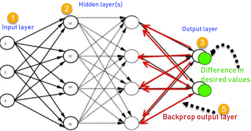
Figure 3.1: Backpropagation Network Architecture - Shows 3-layer network with Input Layer, Hidden Layer(s), and Output Layer. Forward pass computes outputs (→), backward pass propagates errors (←) to update weights.
Components:
1. Input Layer:
- Receives input features
- No computation, just passes data
- Number of neurons = number of features
2. Hidden Layer(s):
- One or more layers
- Performs non-linear transformations
- Extracts features automatically
- Number of neurons is hyperparameter
3. Output Layer:
- Produces final predictions
- Number of neurons = number of classes (classification)
- Or 1 neuron (regression)
4. Connections:
- Fully connected (each neuron connects to all in next layer)
- Each connection has a weight
- Weights are learned during training
5. Activation Functions:
- Hidden layers: Sigmoid, tanh, ReLU
- Output layer: Sigmoid (binary), Softmax (multi-class), Linear (regression)
3.3 Notation
Layers:
- L = total number of layers
- l = current layer (l = 1, 2, ..., L)

Neurons:
- nₗ = number of neurons in layer l
- aᵢˡ = activation of neuron i in layer l

Weights:
- wᵢⱼˡ = weight from neuron j in layer (l-1) to neuron i in layer l

Bias:
- bᵢˡ = bias of neuron i in layer l

Net Input:
- zᵢˡ = weighted sum for neuron i in layer l
- zᵢˡ = Σⱼ wᵢⱼˡ aⱼˡ⁻¹ + bᵢˡ

Activation:
- aᵢˡ = f(zᵢˡ)
3.4 Forward Propagation
Process:
Step 1: Input Layer
    a⁰ = x  (input pattern)

Step 2: For each hidden layer l = 1 to L-1:
    For each neuron i in layer l:
        zᵢˡ = Σⱼ wᵢⱼˡ aⱼˡ⁻¹ + bᵢˡ
        aᵢˡ = f(zᵢˡ)

Step 3: Output Layer (l = L):
    For each output neuron i:
        zᵢᴸ = Σⱼ wᵢⱼᴸ aⱼᴸ⁻¹ + bᵢᴸ
        yᵢ = f(zᵢᴸ)

Step 4: Output y
Example: 2-2-1 Network
Input: x = [0.5, 0.8]
Weights: w₁ = [[0.1, 0.2], [0.3, 0.4]]
         w₂ = [[0.5], [0.6]]
Bias: b₁ = [0.1, 0.2], b₂ = [0.3]

Hidden Layer:
h₁ = sigmoid(0.1×0.5 + 0.2×0.8 + 0.1) = sigmoid(0.31) = 0.577
h₂ = sigmoid(0.3×0.5 + 0.4×0.8 + 0.2) = sigmoid(0.67) = 0.662

Output Layer:
y = sigmoid(0.5×0.577 + 0.6×0.662 + 0.3) = sigmoid(0.986) = 0.728
3.5 Backward Propagation (Error Backpropagation)
Process:
Step 1: Calculate Output Error
    For each output neuron i:
        δᵢᴸ = (tᵢ - yᵢ) × f'(zᵢᴸ)

    Where:
    - tᵢ = target output
    - yᵢ = actual output
    - f'(zᵢᴸ) = derivative of activation

Step 2: Propagate Error Backward
    For each hidden layer l = L-1 down to 1:
        For each neuron i in layer l:
            δᵢˡ = f'(zᵢˡ) × Σₖ wₖᵢˡ⁺¹ δₖˡ⁺¹

    This propagates error from layer l+1 to layer l

Step 3: Calculate Gradients
    For each weight wᵢⱼˡ:
        ∂E/∂wᵢⱼˡ = δᵢˡ × aⱼˡ⁻¹

    For each bias bᵢˡ:
        ∂E/∂bᵢˡ = δᵢˡ

Step 4: Update Weights
    wᵢⱼˡ(new) = wᵢⱼˡ(old) - α × ∂E/∂wᵢⱼˡ
    bᵢˡ(new) = bᵢˡ(old) - α × ∂E/∂bᵢˡ
3.6 Backpropagation Training Algorithm
Complete Algorithm:
Step 1: Initialize
    Set all weights to small random values
    Set learning rate α
    Set maximum epochs

Step 2: For each epoch:
    For each training pattern (x, t):

        # Forward Pass
        Step 2a: Propagate input forward
            Calculate activations for all layers
            Get output y

        # Calculate Error
        Step 2b: Compute error
            E = ½ Σ(tᵢ - yᵢ)²

        # Backward Pass
        Step 2c: Calculate output layer error
            δᵢᴸ = (tᵢ - yᵢ) × f'(zᵢᴸ)

        Step 2d: Backpropagate error
            For each hidden layer (backward):
                δᵢˡ = f'(zᵢˡ) × Σₖ wₖᵢˡ⁺¹ δₖˡ⁺¹

        # Update Weights
        Step 2e: Update all weights and biases
            wᵢⱼˡ = wᵢⱼˡ - α × δᵢˡ × aⱼˡ⁻¹
            bᵢˡ = bᵢˡ - α × δᵢˡ

Step 3: Check Convergence
    If error < threshold OR max epochs:
        Stop
    Else:
        Continue

Step 4: Return trained network
3.7 Testing Process
Testing Algorithm:
Step 1: Load trained weights and biases

Step 2: For each test pattern x:

    Step 2a: Forward Propagation
        Input layer: a⁰ = x

        For each layer l = 1 to L:
            For each neuron i:
                zᵢˡ = Σⱼ wᵢⱼˡ aⱼˡ⁻¹ + bᵢˡ
                aᵢˡ = f(zᵢˡ)

        Output: y = aᴸ

    Step 2b: Make Prediction
        For classification:
            predicted_class = argmax(y)
        For regression:
            predicted_value = y

Step 3: Evaluate Performance
    Calculate accuracy, precision, recall, etc.
Key Difference from Training:
- No backward propagation
- No weight updates
- Only forward pass
- Much faster than training
3.8 Example: Backpropagation
Problem: Train XOR function using 2-2-1 network.
XOR Truth Table:
| x₁ | x₂ | t |
|---|---|---|
| 0 | 0 | 0 |
| 0 | 1 | 1 |
| 1 | 0 | 1 |
| 1 | 1 | 0 |
Network: 2 inputs → 2 hidden → 1 output
Initial Weights (random):
w₁ = [[0.5, 0.5], [0.5, 0.5]]  (input to hidden)
w₂ = [[0.5], [0.5]]             (hidden to output)
b₁ = [0, 0]
b₂ = [0]
α = 0.5
Training Pattern: x = [0, 1], t = 1
Forward Pass:
Hidden layer:
h₁ = sigmoid(0.5×0 + 0.5×1 + 0) = sigmoid(0.5) = 0.622
h₂ = sigmoid(0.5×0 + 0.5×1 + 0) = sigmoid(0.5) = 0.622
Output layer:
y = sigmoid(0.5×0.622 + 0.5×0.622 + 0) = sigmoid(0.622) = 0.651
Error:
E = ½(1 - 0.651)² = 0.061
Backward Pass:
Output layer error:
δ_out = (t - y) × y × (1 - y)
δ_out = (1 - 0.651) × 0.651 × (1 - 0.651)
δ_out = 0.349 × 0.651 × 0.349 = 0.079
Hidden layer errors:
δ_h1 = h₁ × (1 - h₁) × (w₂₁ × δ_out)
δ_h1 = 0.622 × 0.378 × (0.5 × 0.079) = 0.0093

δ_h2 = h₂ × (1 - h₂) × (w₂₂ × δ_out)
δ_h2 = 0.622 × 0.378 × (0.5 × 0.079) = 0.0093
Update Weights:
w₂₁ = 0.5 + 0.5 × 0.079 × 0.622 = 0.525
w₂₂ = 0.5 + 0.5 × 0.079 × 0.622 = 0.525

w₁₁₁ = 0.5 + 0.5 × 0.0093 × 0 = 0.5
w₁₁₂ = 0.5 + 0.5 × 0.0093 × 1 = 0.505
... (and so on)
After many epochs, the network learns XOR!
3.9 Characteristics of Backpropagation
Advantages:
✅ Can solve non-linearly separable problems (XOR)
✅ Learns complex patterns
✅ Automatic feature extraction
✅ Universal function approximator
✅ Foundation for deep learning
Disadvantages:
❌ Slow training (many iterations)
❌ Can get stuck in local minima
❌ Requires careful hyperparameter tuning
❌ Vanishing/exploding gradient problem
❌ Overfitting risk
Solutions:
- Use momentum
- Adaptive learning rates (Adam, RMSprop)
- Batch normalization
- Dropout regularization
- Better initialization (Xavier, He)
Quick Revision Points
Learning Types:
| Type | Data | Feedback | Goal |
|---|---|---|---|
| Supervised | Labeled | Correct answer | Learn mapping |
| Unsupervised | Unlabeled | None | Find patterns |
| Reinforcement | Interaction | Reward/penalty | Maximize reward |
Learning Algorithms:
Hebbian Learning:
Δw = η × x × y
"Neurons that fire together, wire together"
Gradient Descent:
Δw = -α × ∂E/∂w
Move in direction of steepest descent
Delta Rule:
Δw = α × (t - y) × f'(net) × x
Generalized perceptron for continuous functions
Competitive Learning:
Winner-takes-all
Only winner updates: Δw = α × (x - w)
Backpropagation:
Forward Pass:
z = Σ(w × a) + b
a = f(z)
Backward Pass:
Output: δᴸ = (t - y) × f'(z)
Hidden: δˡ = f'(z) × Σ(w × δ)
Weight Update:
w = w - α × δ × a
Expected Exam Questions
15 Marks Questions:
- Explain different types of learning with examples
- Derive Gradient Descent algorithm
- Explain Generalized Delta Rule in detail
- Compare Gradient Descent with Delta Rule
- Backpropagation architecture, training, and testing
- Competitive learning with applications
2.5 Marks Questions:
- Define Supervised/Unsupervised/Reinforcement Learning
- Generalized Delta Learning Rule
- Backpropagation Network
- Competitive Learning
- Separability limitations in unsupervised learning
Derivation Questions:
- Derive Gradient Descent weight update formula
- Derive backpropagation error terms
- Show chain rule application in backpropagation
These notes were compiled by Deepak Modi
Last updated: December 2025